Part 7 investigated signals of two frequencies with sinusoidal phase shift. For the most part, the sample frequency and data time length were constant; only the signal frequencies changed. Not unexpectedly, the lower frequencies were less affected by filter attenuation that were the higher frequencies which approached both the filter corner frequency and the Nyquist limit. At the end of Part 7, I briefly looked at the effect of lessening the sample length. It did not improve the results of the analysis.
In this section, I want to examine the effect of changing the sample rate … which would be the same as maintaining the sample rate and lowering the signal frequencies with respect to the filter corner. I like to recommend a 1st-pass design start with a sample frequency at least 1 decade above the filter corner … and preferably a factor of 20 – 50x for critical applications. This has the disadvantage of opening the noise bandwidth … but design is like squeezing a balloon. Squeeze too hard in one place and something pops out of spec in another. There are other methods for lowering noise – and there are other somewhat lesser known filters which may be suitable for anti-aliasing applications.
I’ve heard it suggested that digital filters are “better” for anti-aliasing. I’m not sure how to apply a digital filter to an analog signal before the signal is quantized …
The signal being used is of the form: F(t) = ½ [sin(2π f1 t + φ) + sin(2π f2 t + φ) ] where φ is identical for and independent of the signal frequencies. The first examination will have the two frequencies at ω1 = 0.83 and ω2 = 0.90 with a sample rate of 47 and data length of 5003. The phase will be set to zero. These are similar in nature to the last plots of Part 7.
The signals with respect to the filter cut-off is the same as it has been in previous sections. Changing the sample frequency does not change this relationship whereas lowering the signal frequency with respect to the filter cut-off has a different effect. Recall that the filters used are 4th-order structures. Typically, these would require 2 opamps, 4 resistors, and 4 capacitors. Performance characteristics would be less for 2nd-order filters.

I’ve shown this plot before. The two signal frequencies are well within the attenuation range of the filters but below the Nyquist frequency. Even an ideal signal is significantly attenuated by the ideal filter.

This has also been shown before. Although the two signal frequencies are at the near-maximum group delay of the Butterworth filter, the delay is roughly equal for both. The Bessel delay is unity but in this example, the important factor is both filters have equal delay for the two signal frequencies.
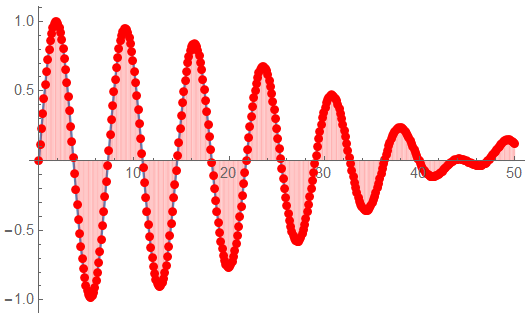
The signal waveform has been shown before but the effect of 47 samples per cycle vs. 2 samples per cycle is pronounced.

The data signal to be analyzed. Slight differences in response are visible.
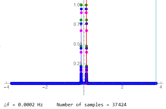
The resulting spectrum. The signals (RED lines) are well below the Nyquist frequency (CYN line) but the signals themselves are hard to distinguish at this scale.

The full-scale positive half plot isn’t an improvement in visualizing the result.

The frequencies are very well distinguished at this scale. The attenuation effects of the filters are visible in the magnitudes. These signal frequencies are too close to the filter cut-off.

The full range phase spectrum. There is no phase factor in these signals (φ = 0)

Phase spectrum detail.
The next example will maintain the sample characteristics but lower each frequency by a factor of 10: ω1 = 0.083 and ω2 = 0.090. Will a sample length of 5003 be sufficient in the “real world”?
Quick math:
Frequency in Hz is ω ÷ 2π = 13.2 mHz. This has a period of 1/f = 75.7 sec. At 47 samples per cycle, a data length of 5003 contains 106 cycles. This should be sufficient. However, 106 cycles at 76 sec/cycle is 8000 sec. If the filter cut-off is de-normalized to 1e6 rad/s, f1 → 13.2 kHz with period of 75.7 μs. 106 cycles would give a data time length of 8 ms.
Allowing for settling time and other factors, a data period of 10 ms collects data at a 100 Hz rate … or 100 data sets per sec. Not unrealistic.
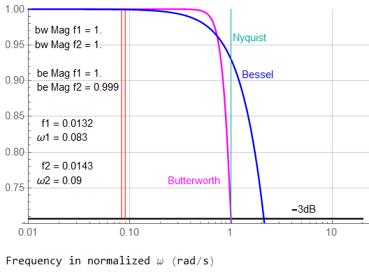
These frequencies seem to be at the upper edge of being affected by filter attenuation. This should be good.

The group delays are constant between these frequencies.

A segment of time data shows virtually no difference between the input and filtered responses … at least at this scale.

A short segment of time data with lots of sample points.

This spectrum plot actually has three responses shown in different colors. BLU is the Bessel response and shows because it was the last set of data specified. At this scale, there appears to be no overlap in response – the filters have no effect on the signal (which is the performance expected of an ideal anti-aliasing filter).

Even at the zoomed-in detail scale, there is no visible difference in responses (the input signal would show as GRN)

A bit of difference shows on the phase spectrum. Both magnitude and phase results are necessary to properly study the analysis results.

The differences in response are visible but appear to be constant in relation to each other. The Butterworth response (MAG) has the longest group delay – at this scale, approximately 2.5x that of the Bessel.
Is the difference important?
The previous sections mostly used a sample frequency twice that of the filter corner and frequencies within 1 decade of that corner. These parameters were based on an actual project … but I want to compare those results to frequencies more than 1 decade below the corner.
I’ll use the sample rate of the previous sections – 2 rad/s – and keep the data length at 5003. The frequencies remain at ω1 = 0.083 and ω2 = 0.090 as in the previous example.
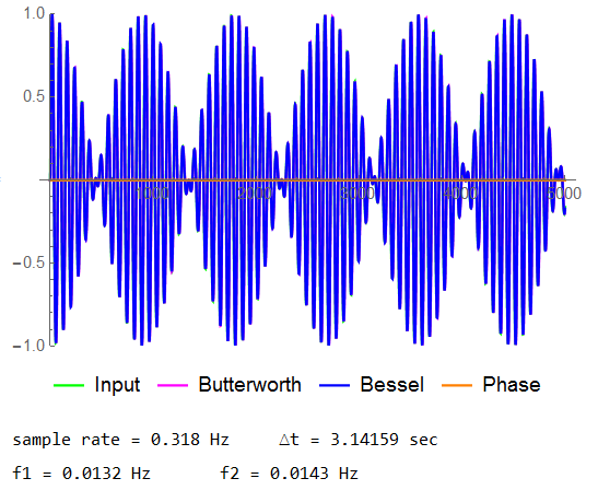
The data segment to be analyzed is 5003 samples long. There is a very distinct beat frequency but no noticeable difference between responses.

The differences due to group delay are still visible though.

The positive spectrum doesn’t show much other than the signal is well below Nyquist.

Looking at the detailed spectrum shows some interaction. Lowering the frequencies by a factor of 10 also lowered the separation by a factor of 10.
Differences in magnitude response aren’t visible even at this scale – the filters have no effect on the signal.

There are noticeable differences in the phase spectrum though

But those differences appear minor in the vicinity of the signal frequencies.
Last plot. I almost promise.
I want to check the low end of the signal range (ω1 = 0.01, ω2 = 0.017) while increasing the data length to 10,007 samples. I’ll keep the sample rate still 2 rad/s.

The signals are now about 2 decades below the filter cut-off and have no effect on the amplitude to at least five 9s. (1.00000 vs. 0.99999)
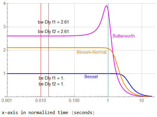
There is no difference in group delay to five places from ω = 0.
BW,dc ⇒ 2.6131326
BW,ω2 ⇒ 2.6131329
BE,dc ⇒ 1.0000000
BE,ω2 ⇒ 1.0000000

The time segment of 10,007 samples

At these frequencies, there is no apparent difference in responses and the calculated magnitude for each frequency is 0.999998 as opposed to the ideal value of 1.000000.
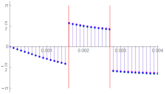
The differences in the phase spectrum are visible in one looks closely

Gridlines are at π/12 intervals – the equivalent of 60°.
Let’s look at the difference in phase at f1:
Signal (GRN): 1.78643 rad → 102.36°
Butterworth (MAG): 1.81267 rad → 103.86°
Bessel (BLU): 1.79647 rad → 102.93°
Seems to be a bit of picking at nits …
Had enough plots yet? … I’ll wrap it up next time.
That’s good for now …
![]()