Filtering – Part 5

To this point, I’ve been considering single-frequency sine waves but most signals consist of a “sum-of-sines”. Within this sum of sines, it is not uncommon for the phase relationships to be random with respect to each other. This can cause difficulty in making amplitude measurements.

Consider this signal:

The summation of two identical sine waves – perhaps from two exactly identical signal sources; each having function 1/2 sin[ω t] with ω = 1/2:

Hard to differentiate the two, eh?

But if the phase of one changes, so does the signal amplitude. The in-phase amplitude is shown in dark green; the out-of-phase signal is shown in light green. The phase angle for this illustration is an arbitrary -2.43 rad; it possibly could vary between radians.

A phase shift of will result in a signal amplitude of zero.

This would be an unusual situation however – more often, even “identical” sources will have slight signal differences.

After filtering, the output (of the lighter green signal) appears as:

Note the delay effects at the beginning of the responses …

 

Consider the sum of two sine waves, one at ω1 = 0.5, the other at ω2 = 0.7 – towards the upper end of the signal band but not unreasonably so given a cut-off frequency of ωc = 1. The phase relationship of ω2 to ω1 is random and may vary between – and +.

A static representation of the signal with the effects of filtering appears as:

But this doesn’t really explain the situation …

 

This plot (in GRN) is the ideal input signal of the sum-of-sines described above. Signal ω1 is the reference; the animated plot shows the variation as the phase shift of Signal ω2 varies from – to +. With a random phase relationship, any one of these amplitudes maybe measured at any given measurement time. Is this important? Could be – depends on the goal of the measurement.

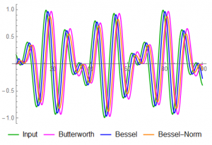
The next three plots show the 4th-order filter responses: MAG is the Butterworth, BLU the standard Bessel, ORG the normalized Bessel. Individually, there’s little obvious difference.

 

The phase differences are apparent when the plots are super-imposed. At ω = 0.5, the Butterworth delay is 2.98, the Bessel delay is 1.00, and the frequency-normalized Bessel is 2.11. At ω = 0.7, the Butterworth delay is 3.51, the Bessel delay is 1.00, and the frequency-normalized Bessel is 2.11.

This is not an illustration of wave propagation; the waves are spatially static, the only change is relative phase for .

The filters are scaled to ω = 1 – although the actual units don’t matter as the scaling between rad/s and Hz is linear via 2π. This is an issue only when time is considered. With proper scaling, the time scale of 100 units would be seconds, however, as shown, the 100 units of time along the x-axis actually represents just shy of 16 s (100 ÷ 2π  =  15.916).

So which filter output is useful for determining amplitude? And how many cycles need to be sampled to obtain an “accurate” measure?

It depends.

 

There are 7.96 cycles of Signal ω1 at ω = 0.5; 11.14 cycles at ω = 0.7.

A 16s segment of  ω  =  0.5 ( sin[ ω1 t ] + sin [ ω2 t ] ) with no phase shift appears as:

Both signals have peak amplitude of 1; the factor of 0.5 puts the peak sum magnitude at 1..

 

Here’s where I have to adjust between rad/s and Hz. The filter cut-off frequency is given as “1” with no specific units given; however, by definition, the frequency ω = 1 rad/s. The sample rate is 2 rad/s. Time being defined as 1/f and noting that f  =  ω/2π, the sample period is 1/π. And we come to a mathematical “quirk”.

Assume an ideal signal frequency of 1 with a sample frequency of 2.

The signal with sample points indicated with RED dots:

Mathematically, there is no frequency content in this signal – and the average value is zero. An unrealistic anomaly. Personally, I try to use prime numbers for sample rates and test frequencies … minimizes harmonic issues.

Page 4
Page 6

That’s good for now …