Distributed Parameters 7 – Transient & Frequency Response

It’s time to consider the transient and frequency response of this network:

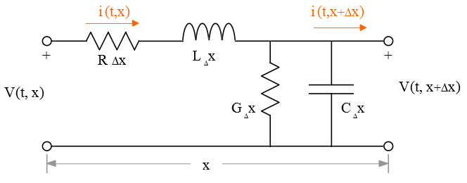
The transform voltage along the line in terms of the transform voltage at the input is given as:

$\begin{displaymath}V(s,x)\;=\;V_o(s,0)\,\frac{\,\mathit{sinh}\Gamma(d-x)\,}{\mathit{sinh}\Gamma d}\quad\textnormal{where:}\;\;\Gamma\;=\;\sqrt{\,(\,L\,s\,+\,R\,)\,(\,C\,s\,+\,G\,)\,}\end{displaymath}$

Apply a unit-step impulse where V_o(s) = s^-1

$\begin{displaymath}V(s,x)\;=\;V_o(s,0)\,\frac{\,\mathit{sinh}\Gamma(d-x)\,}{s\,\mathit{sinh}\Gamma d}\end{displaymath}$

The only singularities are the poles of V(s,x) which are located at s = 0. The roots of sinh(Γd) = 0 come from:

$\begin{displaymath}\Gamma \;=\;\pm\mathit{j}\,k\,\frac{\pi}{\,d\,}\end{displaymath}$

$\begin{displaymath}\begin{align}\textnormal{Define:}\;\;\Gamma\;=\;\sqrt{\,(\,L\,s\,+\,R\,)\,(\,C\,s\,+\,G\,)\,}\;&=\;\sqrt{\,L\,C\,}\,\sqrt{\,(s\,+\,\alpha\,)^2\,-\,\beta\,}\\\\\textnormal{where:}\;\;\alpha\;=\;\frac{1}{\,2\,}\,\left(\,\frac{\,R\,}{L}\,+\,|frac{\,G\,}{C}\,\right)\;\;&\textnormal{and}\;\;\beta\;=\;\frac{1}{\,2\,}\,\left(\,\frac{\,R\,}{L}\,-\,|frac{\,G\,}{C}\,\right)\end{align}\end{displaymath}$

Combining equations gives:

$\begin{displaymath}L\,C\,\left[\,\left(\,s\,+\,\alpha\,\right)^2\,-\,\beta^2\,\right]\;=\;-\frac{\,k^2\,\pi^2\,}{d^2}\qquad\textnormal{where:}\;\;s\;=\;-\alpha\,\pm\,\sqrt{\,\beta^2\,-\,\frac{k^2\,\pi^2}{\,d^2\,L\,C\;}\,}\end{displaymath}$

The poles are complex for large k, may be negative real for small k

Generalizing the pole locations:

$\begin{displaymath}s\;=\;\alpha \,\pm\,\mathit{j}\,\omega_k\qquad\textnormal{where}\;\;\omega_k\;=\;\sqrt{\,\frac{k^2\,\pi^2}{\,d^2\,L\,C\;}\,-\,\beta^2\,}\,\bigg|_{k=1,2,3,...}\end{displaymath}$

The inverse Laplace Transform is found using the residue theorem.

For t > 0:

$\begin{displaymath}v(t,x)\;=\;\sum\,\mathit{res}\,\left[\,\frac{\,\mathit{sinh}\Gamma\,(d-x)\,}{s\,\mathit{sinh}\Gamma d}\,\mathit{e}^{st}\,\right]\end{displaymath}$

which leads to:

$\begin{displaymath}v(t,x)\;=\;\left[\,\frac{\,\mathit{sinh}\Gamma\,(d-x)\,}{s\,\mathit{sinh}\Gamma d}\,\mathit{e}^{st}\,\right]_{s=0}\;+\;\sum_{k=1}^\infty\,\left[\,\frac{\,\mathit{sinh}\Gamma\,(d-x)\,}{s\,\dfrac{d}{d s}\left(\mathit{sinh}\Gamma d\,\right)\,}\,\mathit{e}^{st}\,\right]_{s=-\alpha\pm\mathit{j}\omega_k}\end{displaymath}$

At s = 0, $\Gamma\;=\;\sqrt{\,R\,G\;}$
At s = -α + j ω_k:

$\begin{displaymath}\begin{align}\dfrac{d}{d s}\left(\mathit{sinh}\Gamma d\,\right)\;&=\;d\,\mathit{cosh}\Gamma \,d\,\Frac{\,d\Gamma\,}{d s}\\\\&=\;d\,L\,C\,\mathit{cosh}(\mathit{j}\,k\,\pi)\,\frac{\mathit{j}\,\omega_k}{\mathit{j}\,\dfrac{k\,\pi\,}{d}\,}\\\\&=\;\frac{\;(-1)^k\,\omega_k\,d^2\,L\,C\;}{k\,\pi}\end{align}\end{displaymath}$

From $\mathit{sinh}\Gamma d\;=\;0\,-\,(-1)^k\,\mathit{j}\,\mathit{sin}\left(\,\dfrac{\,k\,\pi\,}{d}\,x\,\right)$

$\begin{displaymath}\left[\,\frac{\,\mathit{sinh}\Gamma\,(d-x)\,}{s\,\dfrac{d}{d s}\left(\mathit{sinh}\Gamma d\,\right)\,}\,\mathit{e}^{st}\,\right]_{s=-\alpha\pm\mathit{j}\omega_k}\;\;=\;\;\frac{k\,\pi\,\left(\,\dfrac{\,k\,\pi\,x\,}{d}\,\right)}{\,d^2\,L\,C\,\omega_k\,\sqrt{\,\omega_k\,+\alpha\,}\,}\,\mathit{e}^{-\mathit{j}\,\Theta}\qquad \textnormal{where:}\;\;\Theta \,=\;\mathit{tan}^{-1}\frac{\alpha}{\,\omega_k\,}\end{displaymath}$

Finally coming to the solution:

$\begin{displaymath}v(t,x)\;=\;\frac{\,\mathit{sinh}\sqrt{\,R\,G\,}\,(d\,-\,x)\,}{d\,\mathit{sinh}\sqrt{\,R\,G\,}}\,-\frac{\,2\,\pi\,\mathit{e}^{-\alpha t}\,}{d^2\,L\,C}\;\sum_{k=1}^\infty\,\frac{\,k\,\pi\,\mathit{sin}\left(\dfrac{\,k\,\pi\,x\,}{d}\,\right)\,}{\omega_k\sqrt{\,\omega_k\,+\,\alpha\,}}\,\mathit{cos}\left(\,\omega_k\,t\,-\,\mathit{tan}^{-1}\frac{\alpha}{\,\omega_k\,}\,\right)\end{displaymath}$

The first term is the steady-state solution; the second is the transient solution.

If the line is a lossless LC network; i.e., R = G = 0

$\begin{displaymath}\textnormal{If}\;\alpha\;=\;\beta\;&=\;0 \qquad s\;&=\;\pm\mathit{j}\,\omega_k\;=\;\pm\mathit{j}\frac{k\,\pi}{\,d\,\sqrt{\,L\,C\,}\,}\end{displaymath}$

giving the solution:

$\begin{displaymath}v(t,x)\;=\;\frac{\,d-x\,}{d}\,-\,\frac{2\,\pi}{\,d^2\,L\,C\,}\,\sum_{k=1}^\infty\,\frac{\,k\,\mathit{sin}\left(\dfrac{\,k\,\pi\,x\,}{d}\,\right)\,}{\omega_k^2}\,\mathit{cos}(\omega_k\,t)\end{displaymath}$

Now consider a distributed RC network; i.e., L = G = 0 stimulated by a unit-step input. Although the above derivation may be used, consider the following:

The transform of the voltage across the network as a function of position is given as:

$\begin{displaymath}V(s,x)\;=\;V(s,0)\,\frac{\,\mathit{sinh}\Gamma(d-x)\,}{\mathit{sinh}\Gamma d}\qquad\textnormal{where}\;\;\Gamma\;=\;\sqrt{\,R\,C\,s\,}\end{displaymath}$

With a unit-step input:

$\begin{displaymath}V(s,x)\;=\;\frac{1}{\,s\,}\,\frac{\,\mathit{sinh}\Gamma(d-x)\,}{\mathit{sinh}\Gamma d}\;=\;\frac{\,\mathit{sinh}\sqrt{\,R\,C\,s\,}\,(d-x)\,}{s\,\mathit{sinh}d\,\sqrt{\,R\,C\,s\,}}\qquad\textnormal{where}\;\;\Gamma\;=\;\sqrt{\,R\,C\,s\,}\end{displaymath}$

Noting $d\,\sqrt{\,R\,C\,s\,}\;=\;\pm\mathit{j}\,n\,\pi\,\big|_{n=1,2,3,...}$

the roots are located at $s\;=\;-\frac{n^2\,\pi^2}{\,d^2\,R\,C\,}$

A bit of algebraic tweaking gives:

$\begin{displaymath}v(t,x)\;=\;\frac{\,d-x\,}{d}\,-\,\frac{2}{\,\pi\,}\,\sum_{n=1}^\infty\,\frac{1}{\,n\,}\,\;\mathit{sin}\left(\,\dfrac{\,k\,\pi\,x\,}{d}\,\right)\,\mathit{exp}\left(\,-\frac{n^2\,\pi^2}{\,d^2\,R\,C\,}\,t\,\right)\end{displaymath}$

That’s good for now. Next: Lumped Parameter Representation

Leave a Comment Cancel Reply