Distributed Parameters 2 – CascadedNetworks

I left off the last section ready to cascade the ideal transmission line model. The cascaded model appears as:

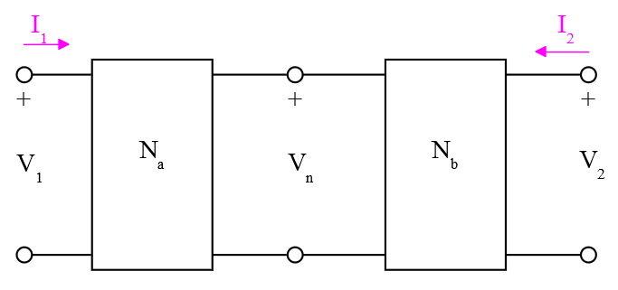
which may be described by:

$\begin{displaymath}\left[ \begin{array}{c}V_1 \\ I_1 \end{array} \right]\;=\;\left[ \begin{array}{cc}A_a & B_a \\ C_a & D_a\end{array} \right]\;\left[ \begin{array}{cc}A_b & B_b \\ C_b & D_b\end{array} \right]\;\left[ \begin{array}{c}V_2 \\ -I_2 \end{array} \right]\;\;\Rightarrow\;\;\left[ \begin{array}{cc}A & B \\ C & D\end{array} \right]\;\left[ \begin{array}{c}V_2 \\ -I_2 \end{array} \right]\end{displaymath}$

where

$\begin{displaymath}\begin{align}A\,=\,A_a\,A_b\,+\,B_a\,C_b&\qquad\qquad B\,=\,A_a\,B_b\,+\,B_a\,D_b\\\\C\,=\,C_a\,A_b\,+\,D_a\,C_b&\qquad\qquad D\,=\,C_a\,B_b\,+\,D_a\,D_b\end{align}\end{displaymath}$

Making substitutions:

$\begin{displaymath}\left[ \begin{array}{c}V(s,d) \\ -I(s,d) \end{array} \right]\;=\;\left[ \begin{array}{cc}\mathit{cosh}\left[\,\Gamma\,\right]\,d & Z_o\,\mathit{sinsh}\left[\,\Gamma\,\right]\,d \\ \frac{\,\mathit{sinh}\left[\,\Gamma\,\right]\,d\,}{Z_o} & \mathit{cosh}\left[\,\Gamma\,\right]\,d\end{array} \right]\;\left[ \begin{array}{c}V(s,0) \\ -I(s,0) \end{array} \right]\end{displaymath}$

where the hyperbolic functions are defined:

$\begin{displaymath}\begin{align}\mathit{sinh}\,\Theta\,&=\,\Theta\,\prod_{n=1}^{\infty}\left(\,1\,-\,\frac{\Theta^2}{\,n^2\,\pi^2\,}\,\right)\\\\\mathit{cosh}\,\Theta\,&=\,\prod_{n=1}^{\infty}\left(\,1\,-\,\frac{4\,\Theta^2}{\,(2\,n-1)^2\,\pi^2\,}\,\right)\end{align}\end{displaymath}$

But it’s so much more convenient to use Mathematica to work through these functions …

The open and short circuit parameters of the uniform transmission line are given as:

$\begin{displaymath}\begin{align}\left[ z_{i,j} \right]\;&=\;\frac{1}{\,Z_o\,}\,\left[ \begin{array}{cc}\mathit{coth}\left[\,\Gamma\,\right]\,d & \mathit{csch}\left[\,\Gamma\,\right]\,d \\ \mathit{csch}\left[\,\Gamma\,\right]\,d & \mathit{coth}\left[\,\Gamma\,\right]\,d\end{array} \right]\;\\\\\left[ y_{i,j} \right]\;&=\;Z_o\,\left[ \begin{array}{cc}\mathit{coth}\left[\,\Gamma\,\right]\,d & \mathit{csch}\left[\,\Gamma\,\right]\,d \\ \mathit{csch}\left[\,\Gamma\,\right]\,d & \mathit{coth}\left[\,\Gamma\,\right]\,d\end{array} \right]\end{align}\end{displaymath}$

The voltage and current expressions of this line having length d as a function of position x are given:

$\begin{displaymath}\begin{align}V(s,x)\,&=\,V(s,d)\,\mathit{cosh}\left[\,\Gamma\,\right]\,(d-x)\,+\,I(s,d)\,Z_o\,\mathit{sinh}\left[\,\Gamma\,\right]\,(d-x)\\\\I(s,x)\,&=\,I(s,d)\,\mathit{cosh}\left[\,\Gamma\,\right]\,(d-x)\,+\,V(s,d)\,\frac{1}{\,Z_o\,}\,\mathit{sinh}\left[\,\Gamma\,\right]\,(d-x)\end{align}\end{displaymath}$

where again, $\Gamma\,=\,\sqrt{\,(\,L\,s\,+\,R\,)\,(\,C\,s\,+\,G\,)\,}$ and

$\begin{displaymath}Z_o\,=\,\sqrt{\,\frac{\,L\,s\,+\,R\,}{\,C\,s\,+\,G\,}\,}\end{displaymath}$

An open-circuit output:

$\begin{displaymath}\begin{align}V(s,x)\,&=\,V(s,0)\,\frac{\,\mathit{cosh}\left[\,\Gamma\,\right]\,(d-x)\,}{\mathit{cosh}\left[\,\Gamma\,\right]\,d}\\\\I(s,x)\,&=\,V(s,0)\,\frac{\,\mathit{sinh}\left[\,\Gamma\,\right]\,(d-x)\,}{Z_o\,\mathit{cosh}\left[\,\Gamma\,\right]\,d}\end{align}\end{displaymath}$

and a short-circuit output:

$\begin{displaymath}\begin{align}V(s,x)\,&=\,V(s,0)\,\frac{\,\mathit{sinh}\left[\,\Gamma\,\right]\,(d-x)\,}{\mathit{sinh}\left[\,\Gamma\,\right]\,d}\\\\I(s,x)\,&=\,V(s,0)\,\frac{\,\mathit{sinh}\left[\,\Gamma\,\right]\,(d-x)\,}{Z_o\,\mathit{sinh}\left[\,\Gamma\,\right]\,d}\end{align}\end{displaymath}$

If a voltage source having impedance Z_S is applied at the input of a line of length d which has a load impedance Z_L

$\begin{displaymath}\begin{align}V(s,x)\,&=\,V(s,0)\,Z_o\,\frac{\,Z_L\,\mathit{cosh}\left[\,\Gamma\,\right]\,(d-x)\;+\;Z_o\,\mathit{sinh}\left[\,\Gamma\,\right]\,(d-x)}{\,Z_o\,(Z_s\,+\,Z_L)\,\mathit{cosh}\left[\,\Gamma\,\right]\,d\,+\,(Z_s\,Z_L\,+\,Z_o^2)\,\mathit{sinh}\left[\,\Gamma\,\right]\,d\,}\\\\I(s,x)\,&=\,V(s,0)\,\frac{\,Z_o\,\mathit{cosh}\left[\,\Gamma\,\right]\,(d-x)\,+\,Z_L\,\mathit{sinh}\left[\,\Gamma\,\right]\,(d-x)}{\,Z_o\,(Z_s\,+\,Z_L)\,\mathit{cosh}\left[\,\Gamma\,\right]\,d\,+\,(Z_s\,Z_L\,+\,Z_o^2)\,\mathit{sinh}\left[\,\Gamma\,\right]\,d\,}\end{align}\end{displaymath}$

This line has no distortion if R/L = C/G

Assume R = G = 0 (zero series resistance; infinite shunt resistance: perfect conductor, perfect insulator – lossless line)

The short-circuit admittance is

$\begin{displaymath}\begin{align}y_{11}\,=\,y_{22}\,&=\,\sqrt{\,\frac{\,C\,}{L}\,}\,\mathit{coth}\left[\,s\,d\,\sqrt{\,L\,C\,}\,\right]\;=\;\frac{1}{\,L\,d\,s\,}\,\prod_{n=1}^\infty\,\left[\,\frac{\,1\,+\,\frac{4\,L\,C\,d^2\,s^2}{\,(2\,n\,-\,1)^2\,\pi^2\,}\,}{1\,+\,\frac{\,L\,C\,d^2\,s^2\,}{n^2\,\pi^2}\,}\,\right]\\\\y_{12}\,=\,y_{21}\,&=\,-\sqrt{\,\frac{\,C\,}{L}\,}\,\mathit{csch}\left[\,s\,d\,\sqrt{\,L\,C\,}\,\right]\;=\;\frac{1}{\,L\,d\,s\,}\,\prod_{n=1}^\infty\,\left[\,\frac{1}{1\,+\,\frac{\,L\,C\,d^2\,s^2\,}{n^2\,\pi^2}\,}\,\right]\end{align}\end{displaymath}$

where the poles and zeroes are located:

$\begin{displaymath}\begin{align}p_o\;&=\;0\\\\p_n\;&=\;\pm\,\mathit{j}\,\frac{n\,\pi}{\,d\,\sqrt{\,L\,C\,}\,}\\\\z_n\;&=\;\pm\mathit{j}\,\frac{\,(2\,n\,-\,1\,)\,\pi\,}{2\,d\,\sqrt{\,L\,C\,}\,}\end{align}\end{displaymath}$

Lumped Parameters

For structures that may be represented with a number of identical sections, an iterated lumped structure can approximate the distributed structure when individual sections are small and the number of identical structures is large.

Consider the T section representation of an incremental lumped parameter network:

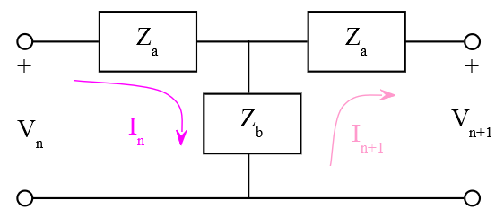
The mesh equations of this network are:

$\begin{displaymath}\begin{align}(Z_a\,+\,Z_b)\,I_n\,-\,Z_b\,I_{n+1}\;&=\;V_n\\\\Z_b\,I_n\,-\,(Z_a\,+\,Z_b)\,I_{n+1}\;&=\;V_{n+1}\quad\textnormal{for}\;n\,=\,0\,\rightarrow\,N-1\end{align}\end{displaymath}$

Re-arranging into matrix form:

$\begin{displaymath}\left[ \begin{array}{c}V_{n+1} \\ I_{n+1}\end{array} \right]\;=\;\left[ \begin{array}{cc}1+\dfrac{Z_a}{Z_b} & -\left(\dfrac{Z_a^2}{Z_b}+2\,Z_a\right) \\ -\dfrac{1}{Z_b} & 1+\dfrac{Z_a}{Z_b}\end{array} \right]\;\left[ \begin{array}{c}V_n \\ I_n \end{array} \right]\end{displaymath}$

Configuring this expression in the form of:

$\begin{displaymath}\left[\,X_{n+1}\,\right]\;=\;\left[\,M\,\right]\,\left[\,X_n\,\right]\;\Rightarrow\;\left[\,X_n\,\right]\;=\;\left[\,M\,\right]^n\,\left[\,X_o\,\right]\end{displaymath}$

The quantity $\left[\,M\,\right]^n$ is found from the eigen values of $\left[\,M\,\right]$ which are found from:

$\begin{displaymath}\textnormal{det}\left|\,M\,-\,\lambda\,I\,\right|\;=\;\lambda^2\,-\,2\,\lambda\,\left(\,\frac{\,Z_a\,}{Z_b}\,+\,1\,\right)\,+\,1\,=\,0\end{displaymath}$

where I is the identity matrix.

The eigen values are related as:

$\begin{displaymath}\lambda_1\,\lambda_2\,=\,1\;\; \textnormal{and}\;\;\lambda_1\,+\,\lambda_2\;=\;2\,\left(\,\frac{Z_a}{\,Z_b\,}\,+\,1\,\right)\end{displaymath}$

Setting $\lambda_1\,=\,\mathit{e}^\tau$ leads to $\lambda_2\,=\,\mathit{e}^{-\tau}$ and $\mathit{cosh}\left[\,\tau\,\right]\;=\;\dfrac{Z_a}{\,Z_b\,}\,+\,1$

Set $M^n\;=\;C_o\,I\,+\,C_1\,M$ which requires:

$\begin{displaymath}\begin{align}\mathit{e}^{\tau n}\,&=\,C_o\,+\,C_1\,\mathit{e}^\tau\\\\\mathit{e}^{-\tau n}\,&=\,C_o\,+\,C_1\,\mathit{e}^{-\tau}\end{align}\end{displaymath}$

Solving for the constants C₀ and C₁:

$\begin{displaymath}C_o\;=\;-\frac{\,\mathit{sinh}[(n-1)\,\tau]\,}{\mathit{sinh}[\tau]}\qquad\textnormal{and}\qquad C_1\;=\;-\frac{\,\mathit{sinh}[n\,\tau]\,}{\mathit{sinh}[\tau]}\end{displaymath}$

A fair bit of pushing and pulling gives

$\begin{displaymath}\left[ \begin{array}{c}V_n \\ I_n\end{array} \right]\;=\;\left[ \begin{array}{cc}\mathit{cosh}[n\,\tau] & -Z_b\,\mathit{sinh}[n\,\tau]\,\mathit{sinh}[\tau] \\ -\dfrac{\mathit{sinh}[\tau]}{Z_b\,\mathit{sinh}[\tau]} & \mathit{cosh}[n\,\tau]\end{array} \right]\;\left[ \begin{array}{c}V_o \\ I_o \end{array} \right]\end{displaymath}$

Since the short-circuit output voltage V_N is 0, the input current is:

$\begin{displaymath}I_o\;=\;\frac{\mathit{cosh}[N\,\tau]}{Z_b\,\mathit{sinh}[N\,\tau]\,\mathit{sinh}[\tau]}\end{displaymath}$

Within the intermediary sections

$\begin{displaymath}\begin{align}I_n\;&=\;V_o\,\frac{\mathit{cosh}[(N-n)\,\tau]}{Z_b\,\mathit{sinh}[N\,\tau]\,\mathit{sinh}[\tau]}\\\\V_n\;&=\;V_o\,\frac{\mathit{sinh}[(N-n)\,\tau]}{\mathit{sinh}[N\,\tau]}\end{align}\end{displaymath}$

Since the open-circuit output current I_N is 0, the input current is:

$\begin{displaymath}I_o\;=\;\frac{\mathit{sinh}[N\,\tau]}{Z_b\,\mathit{cosh}[N\,\tau]\,\mathit{sinh}[\tau]}\end{displaymath}$

Within the intermediary sections

$\begin{displaymath}\begin{align}I_n\;&=\;V_o\,\frac{\mathit{sinh} [(N-n)\,\tau]}{Z_b\,\mathit{cosh}[N\,\tau]\,\mathit{sinh}[\tau]}\\\\V_n\;&=\;V_o\,\frac{\mathit{cosh}[ (N-n)\,\tau]}{\mathit{cosh}[N\,\tau]}\end{align}\end{displaymath}$

For a N-section network:

$\begin{displaymath}\left[ \begin{array}{c}V_N \\ -I_N\end{array} \right]\;=\;\left[ \begin{array}{cc}\mathit{cosh}[N\,\tau] & -Z_b\,\mathit{sinh}[N\,\tau]\,\mathit{sinh}[\tau] \\ -\dfrac{\mathit{sinh}[N\,\tau]}{Z_b\,\mathit{sinh}[\tau]} & \mathit{cosh}[n\,\tau]\end{array} \right]\;\left[ \begin{array}{c}V_o \\ -I_o \end{array} \right]\end{displaymath}$

The short-circuit admittance parameters:

$\begin{displaymath}\begin{align}y_{11}\;=\;y_{22}\;&=\;\frac{\mathit{cosh}[N\,\tau]}{\,Z_b\,\mathit{sinh}[\tau]\,\mathit{sinh}[N\,\tau]\,}\;=\;\frac{\mathit{coth}(N\,\tau)}{\,Z_b\,\mathit{sinh}(\tau)\,}\\\\y_{12}\;=\;y_{21}\;&=\;\frac{-1}{\,Z_b\,\mathit{sinh}[\tau]\,\mathit{sinh}[N\,\tau]\,}\;=\;-\frac{\mathit{csch}[N\,\tau]}{\,Z_b\,\mathit{sinh}[\tau]\,}\end{align}\end{displaymath}$

For ease in pole-zero analysis, it is desired to express these relationships in factored form. Applying the expansions of the hyperbolic functions shown in an earlier post, the admittance parameters can be expressed as::

$\begin{displaymath}\begin{align}y_{11}\;=\;y_{22}\;&=\;\dfrac{\prod_{n=1}^N\left(\,\dfrac{Z_a}{\,Z_b\,}\,+\,1\,-\,\mathit{cos}\left[\,\dfrac{\,(2\,n\,-\,1)\,\pi\,}{2\,n}\,\right]\,\right)}{\;Z_b\,\left[\,\left(\,\dfrac{Z_a}{\,Z_b\,}\,+\,1\,\right)^2\,-\,1\,\right]\,\prod_{n=1}^{N-1}\left(\,\dfrac{Z_a}{\,Z_b\,}\,+\,1\,-\,\mathit{cos}\left[\,\dfrac{\,n\,\pi\,}{N}\,\right]\,\right)}\\\\y_{12}\;=\;y_{21}\;&=\;\dfrac{-1}{\;Z_b\,2^{N-1}\,\left[\,\left(\,\dfrac{Z_a}{\,Z_b\,}\,+\,1\,\right)^2\,-\,1\,\right]\,\prod_{n=1}^{N-1}\left(\,\dfrac{Z_a}{\,Z_b\,}\,+\,1\,-\,\mathit{cos}\left[\,\dfrac{\,n\,\pi\,}{N}\,\right]\,\right)}\end{align}\end{displaymath}$

For a lossless line:

$y_{11}\;=\;y_{22}\;&=\;\dfrac{s\,C\,\prod_{n=1}^N\left(\,1\,-\,\mathit{cos}\left[\,\dfrac{\,(2\,n\,-\,1)\,\pi\,}{2\,n}\,\right]\,+\,\dfrac{\,L\,C\,s^2\,}{2}\,\right)}{\;\left[\,\left(\dfrac{\,L\,C\,s^2\,}{2}\,+\,1\,\right)^2\,-\,1\,\right]\,\prod_{n=1}^{N-1}\left(\,1\,-\,\mathit{cos}\left[\,\dfrac{\,n\,\pi\,}{N}\,\right]\,\right)\,+\,\dfrac{\,L\,C\,s^2\,}{2}\,}$

$\begin{displaymath}Z_a\;=\;\frac{\,L\,s\,}{2}\qquad Z_b\;=\;\frac{1}{\,C\,s\,}\qquad\frac{Z_a}{\,Z_b\,}\;=\;\frac{\,L\,C\,s^2\,}{2}\end{displaymath}$

so that:

$\begin{displaymath}\begin{align}y_{11}\;=\;y_{22}\;&=\;\dfrac{s\,C\,\prod_{n=1}^N\left(\,1\,-\,\mathit{cos}\left[\,\dfrac{\,(2\,n\,-\,1)\,\pi\,}{2\,n}\,\right]\,+\,\dfrac{\,L\,C\,s^2\,}{2}\,\right)}{\;\left[\,\left(\dfrac{\,L\,C\,s^2\,}{2}\,+\,1\,\right)^2\,-\,1\,\right]\,\prod_{n=1}^{N-1}\left(\,1\,-\,\mathit{cos}\left[\,\dfrac{\,n\,\pi\,}{N}\,\right]\,\right)\,+\,\dfrac{\,L\,C\,s^2\,}{2}\,}\\\\y_{12}\;=\;y_{21}\;&=\;\dfrac{-1}{\;2^{N-1}\,\left[\,\left(\dfrac{\,L\,C\,s^2\,}{2}\,+\,1\,\right)^2\,-\,1\,\right]\,\prod_{n=1}^{N-1}\left(\,1\,-\,\mathit{cos}\left[\,\dfrac{\,n\,\pi\,}{N}\,\right]\,\right)\,+\,\dfrac{\,L\,C\,s^2\,}{2}\,}\end{align}\end{displaymath}$

For a distributed RC line,

$\begin{displaymath}Z_a\;=\;\frac{\,R\,}{2}\qquad Z_b\;=\;\frac{1}{\,C\,s\,}\qquad\frac{Z_a}{\,Z_b\,}\;=\;\frac{\,R\,C\,s^2\,}{2}\end{displaymath}$

and:

$\begin{displaymath}\begin{align}y_{11}\;=\;y_{22}\;&=\;\dfrac{s\,C\,\prod_{n=1}^N\left(\,1\,-\,\mathit{cos}\left[\,\dfrac{\,(2\,n\,-\,1)\,\pi\,}{2\,n}\,\right]\,+\,\dfrac{\,R\,C\,s\,}{2}\,\right)}{\;\left[\,\left(\dfrac{\,R\,C\,s\,}{2}\,+\,1\,\right)^2\,-\,1\,\right]\,\prod_{n=1}^{N-1}\left(\,1\,-\,\mathit{cos}\left[\,\dfrac{\,n\,\pi\,}{N}\,\right]\,\right)\,+\,\dfrac{\,R\,C\,s\,}{2}\,}\\\\y_{12}\;=\;y_{21}\;&=\;\dfrac{-C\,s}{\;2^{N-1}\,\left[\,\left(\dfrac{\,R\,C\,s\,}{2}\,+\,1\,\right)^2\,-\,1\,\right]\,\prod_{n=1}^{N-1}\left(\,1\,-\,\mathit{cos}\left[\,\dfrac{\,n\,\pi\,}{N}\,\right]\,\right)\,+\,\dfrac{\,R\,C\,s\,}{2}\,}\end{align}\end{displaymath}$

with simple poles located at:

$\begin{displaymath}s\;=\;-\frac{2}{\,R\,C\,}\,\left[\,1\,-\,\mathit{cos}\left(\frac{\,n\,\pi\,}{N}\,\right)\,\right]_{n=0\,1,\rightarrow N}\end{displaymath}$

That’s good for now. Next: Non-Uniform Distribution

Leave a Comment Cancel Reply