Looking at a page of algebraic derivations and equations is useful – almost as much so as understanding them.
But pictures are pretty … pictures are good. Visualization can be an aid to understanding.
In summary, the two primary noise types appear similar to the following:
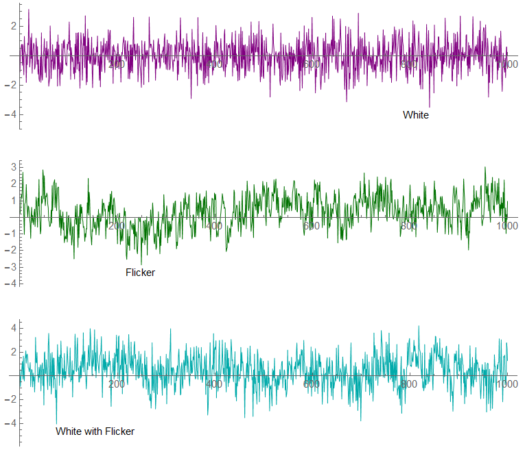
This image is made of 1000 samples.
“Red” Noise
This noise has a power spectrum proportional to 1/f![]() . This is more commonly known as “Drunkard’s Walk” (or “random walk”). This noise can come about through the integration of white noise. In the time-domain, this noise has an appearance somewhat like this (300,000 sample points)
. This is more commonly known as “Drunkard’s Walk” (or “random walk”). This noise can come about through the integration of white noise. In the time-domain, this noise has an appearance somewhat like this (300,000 sample points)
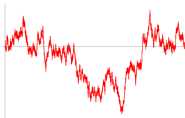
This type of noise does not have a constant variance and averaging will increase the uncertainty. Whereas with white noise, σ![]() is a function of n
is a function of n![]() , with red noise, σ
, with red noise, σ![]() is a function of n
is a function of n![]() .
.
Here’s a representative sample of Gaussian noise.
Mean = 0.0 ; σ = 1 (RMS) ; N = 1000
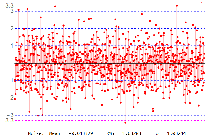
Not quite “perfect” even with 1000 samples. If I were measuring “zero volts”, I’d read an offset of -43 mV. Dashed BLU lines indicate ±1 σ, ±2 σ, ±3 σ, and ±3.3 σ (MAG).
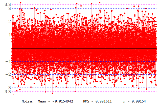
Out of curiosity, I set up a sequence of 10007 samples (a prime number).
Even with this many samples, averaging resulted in an offset of -15 mV.
I’ll now look at some effects of noise on a signal consisting of a single frequency.
Each example will have the same input signal: One period of a sine wave. Peak value 5V. The waveform is riding on a common-mode signal of 10 VDC (so that the magnitude of the waveform is entirely positive). The rms value of the sine wave with no offset is 3.536 V.

The noise representations are defined to have an rms value of 1. Recall the rms value of a Gaussian distribution is 1 standard deviation σ.
The signal-to-noise ratio is: ![]() = 10.61 ⇒ 20.51 dB – an attenuation factor of about 10. This would be my minimum recommended SNR (representing the minimum usable signal – as opposed to the minimum detectable signal).
= 10.61 ⇒ 20.51 dB – an attenuation factor of about 10. This would be my minimum recommended SNR (representing the minimum usable signal – as opposed to the minimum detectable signal).
The only difference in the following plots is the number of samples per period.
The noise is generated with a “white noise process” of mean zero and standard deviation of 1. Each sample is independent with identical distribution. The SNR ratio for all examples is 10.61/1 or 20.5 dB.
The plots are in pairs The mean and rms value of the noise itself and the signal+noise are calculated for each data set.
Note that sample count N is effectively the over-sample factor where N is samples per period. The Nyquist limit would be N = 2. Also note that an ideal sine wave sampled at a Nyquist rate of 2 can result in a DC signal, value 0.
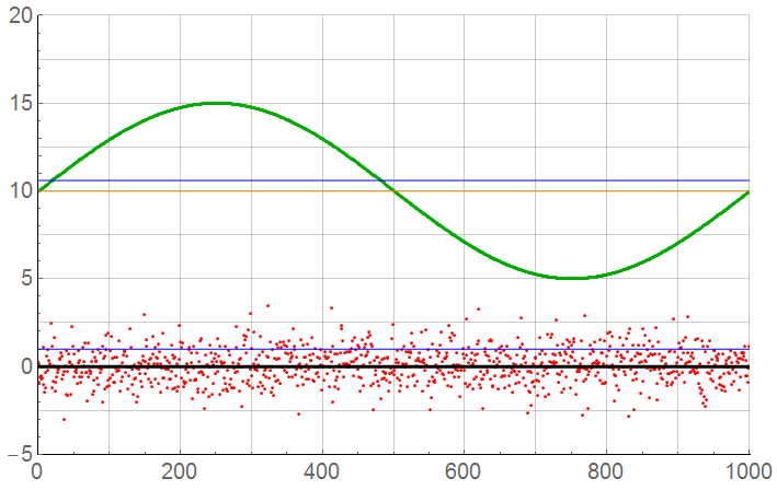
N = 1000
The first plot of the pair shows the ideal sampled signal along with the associated noise. The signal is indicated in GRN; the noise in RED. The BLK line at 0 is the ideal noise mean; the BLU line at 1 is the ideal standard deviation of noise. The ORG line is the DC offset of 10 V; the BLU line is the effective rms value of 10.61 V.
The second plot of each pair adds the noise to the signal. The MAG points are the magnitudes that would actually be digitized. The lower trace is the noise component which would not be part of the measurement. Again, the SNR is 20.5 dB. These patterns hold true for the remaining illustrations. The mean should be 10.00; the rms should be 10.61. σ should be 1.00.
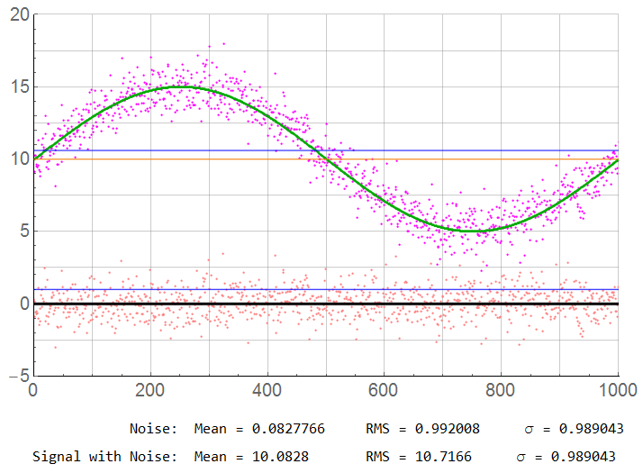
For N = 1000: Although the sample count is high, there is still possibly significant error. The “true” RMS value is 10.61; the mean should be 10.00. There is a 0.83% error … which may be acceptable in many cases. The sample rate is 500x the Nyquist limit.
N = 100
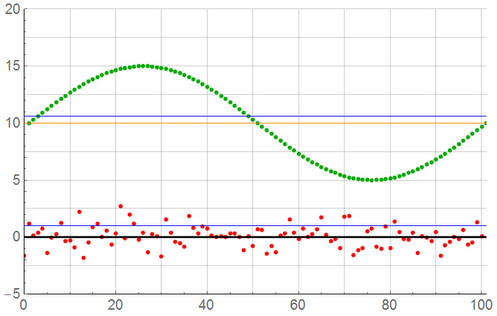
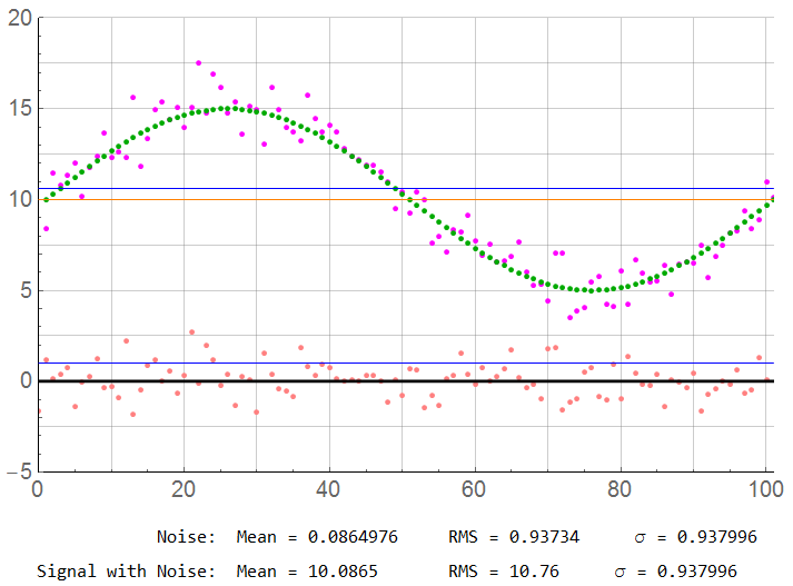
For N = 100: The sample count has been reduced by a factor of 10 but is still high. The error has increased very slightly – but an insignificant amount. The error from mean is now 0.87% … which may still be acceptable. The sample rate is 50x the Nyquist limit. A different data set with identical parameters may give different results.
N = 50
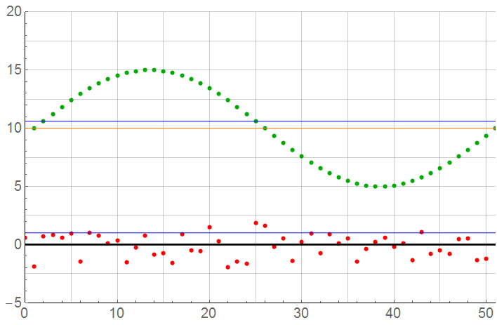
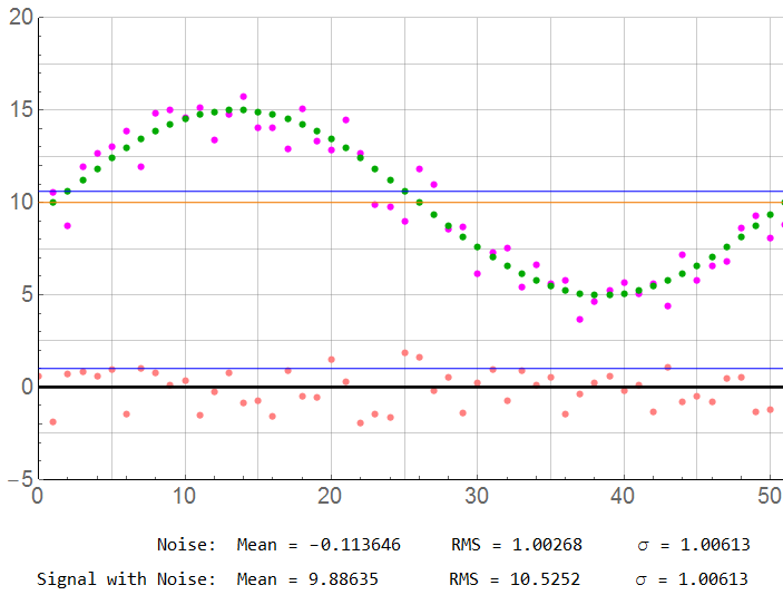
For N = 50: The sample count is now at the point where errors may not be acceptable except for crude measurements. The error from mean has now increased to 1.14% … often acceptable but better classified as “good enough” rather than accurate (for what I define as 1% or better). The sample rate is 25x the Nyquist limit.
N = 20
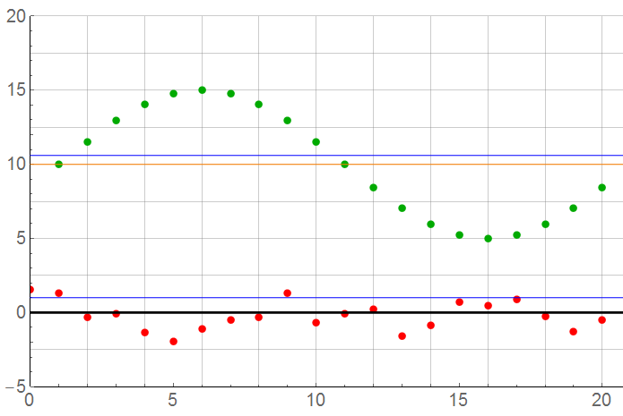
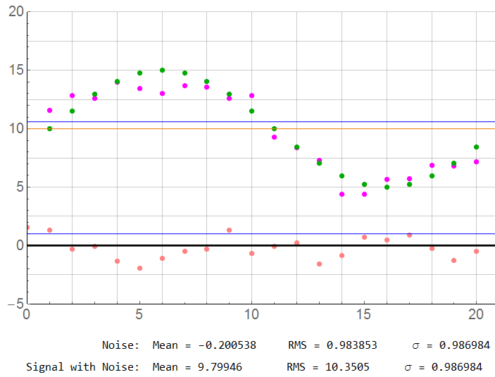
For N = 20: The sample count is now at the point where errors may not be acceptable except for crude measurements. Recall the MAG magnitudes are the measure; the GRN dots are the true value. The error from mean now exceeds 2% … good enough? Possibly. Probably OK for a rough environment field measurement system. The sample rate is 10x the Nyquist limit.
N = 10
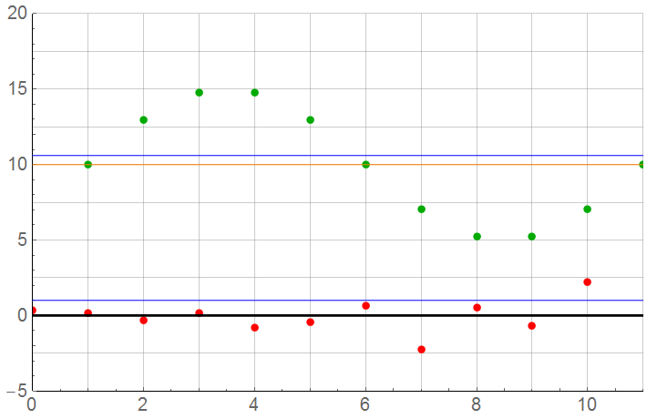
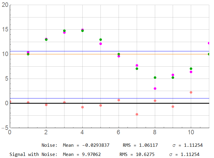
For N = 10: Borderline acceptable but the error from this particular noise set has improved to below 1%. Does this mean a sample rate of 5x Nyquist is acceptable? Recall that a higher sample rate with the same noise characteristics (and more samples averaged) resulted in errors over 2%. One sample set may be acceptably accurate; the next set may not. It would be difficult to properly interpret or develop an accurate inverse model from such data. Each data set would have an overall random error.
On the other hand, these are examples of identical information with the only variation being in independent samples of a Gaussian function – ideal for averaging. For example, I collected 24 data sets of the N = 10 signal+noise sequence. The mean value for the sum of sets was 9.91085 – less than 1% error from the mean (-0.89%). The standard deviation was 0.3367.
24 sequences of 10 samples each. 240 sample points. I also did a single sample sequence with 240 points. The mean was 10.0325 (0.33% error) with a standard deviation of 1.02423.
Consider the differences if I were collecting a single data set for each measurement environment in which that environment changed at every sample … perhaps an airplane taking geophysical measurements over a long flight path. Perhaps the terrain changes slowly (Calgary to Winnipeg) or quickly (Las Vegas to San Francisco).
10 samples per cycle would be the lowest sample rate I’d recommend for general purposes; I’d prefer 20 to 50 samples per cycle.
One last one: N = 3 samples per cycle (where the Nyquist limit is 2 samples per cycle)
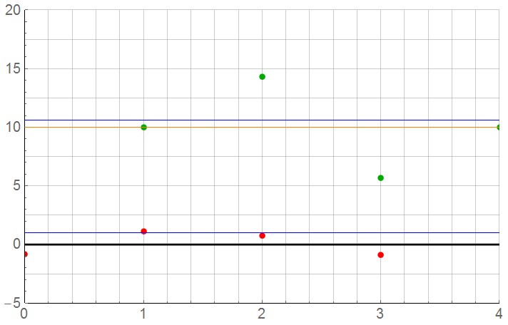
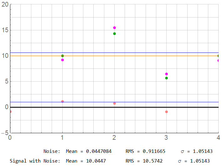
As it turn out, this is one of the more accurate results: The mean is 10.0447 (0.45% error) and standard deviation is 1.05 instead of 1.0.
When I collected a second sequence though, the mean was 9.2846 … an error of -7.2 %.
White noise being stationary allows the assumption that the mean and variance are constant. When this assumption is true, the noise is considered a stationary process.
This first plot is an example of stationary white noise: the mean and variance are constant throughout. Averaging will decrease the variance.
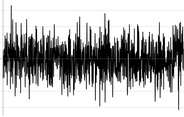
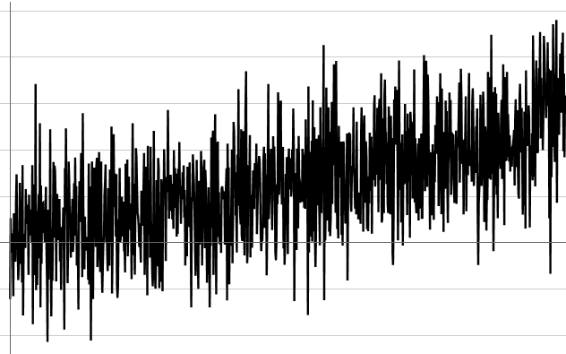
… while the following plot represents non-stationary white noise (if it’s not stationary, is it white noise?).
In this plot, the mean shifts upward over time … or is it due to flicker or burst noise? The criteria for proper averaging is not present.
In this figure, the variance is not constant although the mean remains so.
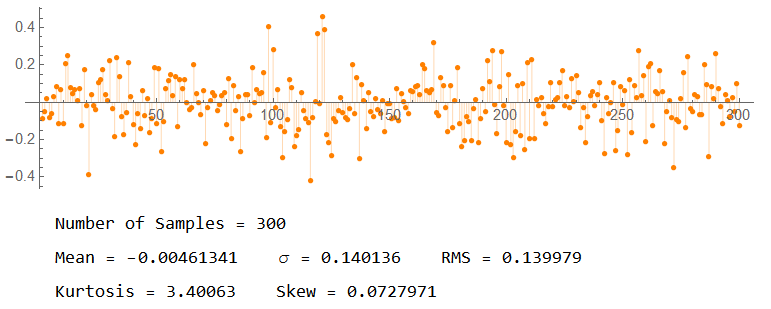
The values of skewness and kurtosis are indicators of the “closeness” to a Gaussian approximation. These values obtained with a sample set size of 300.
This plot shows the effect the previous noise set has on a 1 V sine wave.

The noise is non-stationary with a sample rate of 100 samples per cycle. Low-pass filtering would help here. Such noise would likely be introduced to the signal close to or at the transducer (given proper circuit construction procedures). A low-pass Butterworth filter would be acceptable if the signal frequency were low compared to the filter cut-off; a Thomson filter would be the better choice if phase information were important and/or the signal frequencies were within about 1 decade of the filter corner.
One last note: I didn’t follow my own procedures herein, but I usually like to use prime numbers as a sample rate when I perform integer-based sampling.
That’s all for now.
