ADC Wiggles to Bits 6a Central Limit Theorem and Probability Distributions

Noise does not necessarily decrease by averaging samples, particularly for a small number of samples. Both the Central Limit Theorem and the binomial distribution approximation to normal lose validity as N → 0.

Central Limit Theorem

When discussing small sample sets, assuming a Poisson distribution is often more appropriate than the Gaussian. The Central Limit Theorem is often used as a justification for assuming all noise is treated as Gaussian, but the CLT is based on the assumption of a “large” number of samples – “large” being a somewhat ambiguous term.

“The central limit theorem asserts that means of independent, identically distributed variables will converge to a normal distribution provided they are light-tailed enough. This means that even when the exact distribution is not known for some quantity, if there is some form of averaging process going on you will eventually end up with normal distributions. This is the basis for a long list of statistical decision procedures.“

More formally¹:

Let $\mathbb{X}_1$ , $\mathbb{X}_2$ , … $\mathbb{X}_N$ be a set of N independent random variates and each $\mathbb{X}_i$ have an arbitrary probability distribution $\mathbb{P}(x_i)$ with mean $\mu_i$ and finite variance $\sigma_i^2$ . Then the normal form variate is:

$\begin{displaymath} \mathbb{X}_{\text{norm}} \; \equiv \; \frac{\; \; \sum_{i=1}^N x_i \; - \; \sum_{i=1}^N \mu_i \;}{\sqrt{ \, \sum_{i=1}^N \sigma_i^2 \; } \, } \end{displaymath}$

and has a limiting cumulative distribution function which approaches a normal distribution.

Under additional conditions on the distribution of the addend, the probability density itself is also normal with mean $\mu$ = 0 and variance $\sigma^2$ = 1. If conversion to normal form is not performed, then the variate:

$\begin{displaymath} \mathbb{X} \; \equiv \; \frac{1}{\, N \, } \, \sum\limits_{i=1}^N x_i \end{displaymath}$

is normally distributed with $\mu_{\mathbb{X}} \, = \, \mu_x}$ and $\sigma_{\mathbb{X}} \, = \, \sigma_x/\sqrt{\, N \, }}$

Although this definition requires “identically distributed” samples, another version presented by Liapounov² does not require identical distributions but does require finite mean and variance.

$\, \lim\limits_{N \rightarrow \infty} \, \frac{1}{\, s_n^{2+\delta} \, } \, \sum\limits_{i=1}^n \mathbb{E} \left[ \left|\text{X}_i \, - \, \mu_i \right|^{2+\delta} \, \right] \; = \; 0$

All well and good. Pay attention to the many conditions: “identically-distributed”, “light tailed enough”, “eventually end up with”, “N → ∞”, and most particularly, references to “large enough”. The CLT is an approximation based on large numbers. Electronic noise does not always follow these conditions and a “large number” is not defined.

My concern is the use of averaging. There exists a tendency to use the mathematics of a Gaussian distribution in situations it does not apply – so I need to determine what a suitable “large enough” number is.

Probability Distributions

Uniform Distribution:
All occurrences are constrained to well-defined limits. Any value within those limits has equal probability of occurrence. Tossing a single honest die is a good example: One of six possible outcomes, each outcome having equal probability

Binomial Distribution
Calculates the number of occurrences out of a fixed number of possibilities. Any single occurrence has probability p. The binomial distribution is approximated by a Gaussian distribution as the number of samples increases. The toss of a coin is a common example where it is assumed there are only two possible outcomes (though last time I looked at a coin, it had three surfaces). Probability of state in digital representation of white noise would be another example.

Gaussian Distribution
aka “normal” distribution. The “bell curve”. Commonly used to determine measurement errors. The normal distribution is a Gaussian distribution with mean of zero and variance of 1. A continuous approximation to the discrete binomial distribution for a very large number of samples. The Central Limit Theorem states that the mean of a large set of a variety of individual distributions tends towards a normal distribution … as the number of samples tends towards “very large”. Feller³ suggests a reasonable approximation requires a minimum of 5 samples.

Poisson Distribution
Calculates the number of occurrences within a given interval given the average number of occurrences per interval. Shot noise – photon and electron – has a Poisson distribution. The variance equals the mean. Tends to a binomial distribution as the number of samples increases.

I’ll be mostly concerned with the Gaussian and Poisson distributions – the point being that sample numbers are often not sufficient to make precise measurements based solely on Gaussian-based analyses. Low-frequency and low-level signals come to mind ..

Gaussian Addition and Multiplication

If one Gaussian measure of x $_{\text{1}}$ + σ $_{\text{1}}$ is added to another x $_2$ + σ $_2$ , the sum of these two Gaussian distributions would have a Gaussian mean of x $_{\text{1}}$ + x $_2$ but the distribution of uncertainty would be:

$\begin{displaymath} \sigma_{\text{sum}} \; = \; \sqrt{ \, \sigma_1^2 \, + \, \sigma_2^2 \, + \, ... \; } \end{displaymath}$

If the measures were multiplied, the product would have mean x $_1$ times x $_2$ but the distribution would be:

$\begin{displaymath} x_{\text{prod}} \; = \; x_1 \; x_2 \, \left( \; 1 \, \pm \, \sqrt{ \, \frac{\; \sigma_1^2 \;}{x_1^2} \, + \, \frac{\; \sigma_2^2 \;}{x_2^2} \, + \, ... \; } \; \right) \end{displaymath}$

Skewness and Kurtosis

Skewness is a measure of symmetry while kurtosis is a measure of concentration of data about the mean (fatness of curve). Positive skewness implies data with a longer right-sided tail; negative skewness implies data toward a a longer left-sided tail. Kurtosis greater than 3 implies a “peakiness”; less than 3 indicates “flatness”.

The Gaussian distribution has kurtosis of 3.0 and skewness of 0. For the number of samples N to be “large enough”, the kurtosis and skewness of the resulting Poisson function must approach these values.

The Poisson distribution has kurtosis of 3 + $1/\mu$ with skewness of $1/\sqrt{\mu \,}$ . For 10 samples, kurtosis is 3.1; skewness is 0.316. For 5 samples, kurtosis is 3.2; skewness is 0.447. The Gaussian values are kurtosis of 3.0 and skewness of 0. Data sets of 5 and 10 samples do not fit the criteria of “large enough”.

A Mathematica routine to explore “large” is used:

data[n_] := TransformDistribution[Total[Array[x,n],
Array[x,n] $\approx$ ProductDistribution[{PoissonDistribution[1],n}]]
Table[Skewness[data[n]],{n, 1, 10 001, 1000}]//N
Table[Kurtosis[data[n]],{n, 1, 10 001, 1000}]//N

This routine provides the values for skewness and kurtosis for 1 to 10001 samples by 1000. The results follow:

$\begin{array}{r|cc} \text{\#Samples} & \text{skewness} & \text{kurtosis} \\ \hline 1 & 1.0 & 4.0 \\ 1001 & 0.0316 & 3.0010 \\ 2001 & 0.0224 & 3.0005 \\ 3001 & 0.0183 & 3.0001 \\ 4001 & 0.0158 & 3.0001 \\ 5001 & 0.0141 & 3.0001 \\ 6001 & 0.0129 & 3.0001 \\ 7001 & 0.0120 & 3.0001 \\ 8001 & 0.0112 & 3.0001 \\ 9001 & 0.0105 & 3.0001 \\ 10001 & 0.0100 & 3.0001 \\ \end{array}$

I’d be willing to state that even 1001 samples is a close representation of a normal distribution. Perhaps if I were measuring resistance values in a lab, I could effectively collect even more than 1000 samples … high speed clock and all. But I also suspect I could get by with fewer samples.

So repeat with increments of 100 up to 1000.

$\begin{array}{r|cc} \text{\#Samples} & \text{skewness} & \text{kurtosis} \\ \hline 1 & 1.0 & 4.0 \\ 101 & 0.0995 & 3.0099 \\ 201 & 0.0705 & 3.0050 \\ 301 & 0.0576 & 3.0033 \\ 401 & 0.0499 & 3.0025 \\ 501 & 0.0447 & 3.0020 \\ 601 & 0.0408 & 3.0017 \\ 701 & 0.0378 & 3.0014 \\ 801 & 0.0353 & 3.0013 \\ 901 & 0.0333 & 3.0011 \\ 1001 & 0.0316 & 3.0010 \\ \end{array}$

“Hundreds” gets into the range of “how good does it need to be?”. The shape of the “bell” is good throughout the range but there’s a tendency to emphasize the higher values.

Try again by 10s to 100.

$\begin{array}{r|cc} \text{\#Samples} & \text{skewness} & \text{kurtosis} \\ \hline 1 & 1.0 & 4.0 \\ 11 & 0.3015 & 3.0909 \\ 21 & 0.2182 & 3.0476 \\ 31 & 0.1796 & 3.0323 \\ 41 & 0.1562 & 3.0244 \\ 51 & 0.1400 & 3.0196 \\ 61 & 0.1280 & 3.0164 \\ 71 & 0.1187 & 3.0141 \\ 81 & 0.1111 & 3.0124 \\ 91 & 0.1048 & 3.0110 \\ 101 & 0.0995 & 3.0099 \\ \end{array}$

A little bit extra emphasis towards the mean and skewed a bit high. I need 34 samples before kurtosis gets within 1% of the Gaussian ideal value of 3. Poisson skewness is 0.171 at N = 34. This would tend to over-estimate the mean if Gaussian assumptions are used.

When taking field measurements, it may not be possible to collect more than a couple of samples … and it may not be desirable to do so, but since the tendency is to average everything under the assumption of a Gaussian distribution, let’s see how close a smaller number of samples gets.

$\begin{array}{r|cc} \text{\#Samples} & \text{skewness} & \text{kurtosis} \\ \hline 1 & 1.0 & 4.0 \\ 2 & 0.707 & 3.50 \\ 3 & 0.577 & 3.33 \\ 4 & 0.500 & 3.25 \\ 5 & 0.447 & 3.20 \\ 6 & 0.408 & 3.17 \\ 7 & 0.378 & 3.14 \\ 8 & 0.354 & 3.13 \\ 9 & 0.333 & 3.11 \\ 10 & 0.316 & 3.10 \\ \end{array}$

By making the assumption that mean and variance are known, the use of only a few samples is validated … assuming the assumption is true. Since determining a “mean” is often the point of the measurement, the assumption is not valid.

Although an argument might be made that 10 samples suitably represents a “bell” shape, the skewness (which should be close to zero) is large enough that the assumption of Gaussian characteristics for improvement by averaging is not valid. Furthermore, it is quite likely that field measurements – especially with moving platforms – do not meet the stationary criteria. It would also appear that the Central Limit Theorem allowing samples of disparate distributions to be combined as Gaussian “in the limit” is not valid for such small numbers of samples.

On the other hand, how “valid” do you wish to be? (Possibly more so than this.)
What is the desired accuracy of the results?

Think of it this way. The Poisson distribution is based on positive integers. While there is room to “spread” the tail towards more positive values, there is less room to spread to the less positive values as the number of samples decreases – the distribution gets “squished” at 1 as the number of samples decreases.

Perhaps a few plots would be clearer than a list of numbers:

The Poisson Distribution for 1, 2, 5, and 10 samples. By eye, 10 samples looks close to a Gaussian; the skewness of 0.316 shows it tends fairly strongly to the right with a slight tendency to over-emphasize values to the mean.

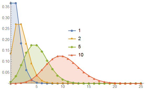
If I were making measurements such as this and using the assumption of Gaussian distribution, I might be inclined to report a mean value a bit higher than the “true” value.

Looking at a comparison to the Gaussian (in RED) shows a not-bad closeness to the bell shape, but the left tail is cut off.

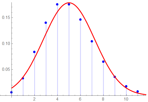
The Gaussian representation is in RED, the measured data is in BLU. Note the truncation at 1 – hard to have fewer than 1 sample …
The skewness of the Gaussian representation is 0.996; the kurtosis is 4.1. Analyzing this data set with Gaussian assumptions is not valid.

Of course, one should note that this distribution has 10 samples – of a stationary system. This may not be feasible with field measurements. The point being that the process of averaging to improve the measurement quality is based on assuming the validity of the Central Limit Theorem, Gaussian probabilities, and a stochastic sample set. These assumptions do not appear to be valid for small numbers of samples … and it may not be feasible to collect a sufficient number to be considered “large”.

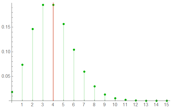
A sample set of 4 is not uncommon. Under Gaussian analysis, averaging 4 samples will reduce the variance by ½. The Poisson distribution mean is the number of “occurrences”. The statistical characteristics are defined by the mean $\mu$ : the variance is equal to the mean, the skewness is 1/ $\sqrt{\mu}$ , and kurtosis is 3 + 1/ $\mu$ .

The first of the following charts shows the Poisson variance for 4 samples;

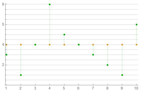
The second shows a possible shift in measure over 10 sets of 4 samples.

That’s good for now.

¹Weisstein, Eric W. “Central Limit Theorem.” MathWorld–A Wolfram Web Resource

²Thomas, John B. “An Introduction to Applied Probability and Random Processes

³Feller, W. “An Introduction to Probability Theory and Its Applications