Distributed Parameters 10 – Coordinate Systems

The determination of non-uniform current flow and equipotential lines of force are aided by the use of other coordinate systems. There are four coordinate systems feasible for 2-d networks: rectangular (Cartesian), polar, parabolic, and elliptic. Expressions are developed for the polar and parabolic systems.

Polar

Consider a polar coordinate system. This geometry represents a linear electrical taper.

In this system, equipotential lines are circles; current flow follows radii. Port 1 will be defined as x = 0; port 2 is at x = d. The coordinate system center is at x = – x₀. The network width is found from:

$\begin{displaymath}w\;=\;\frac{\,\theta\,x_o\,}{2\,\pi}\,\left(\,1\,+\,\frac{x}{\,x_o\,}\,\right)\;=\;w_o\,\left(\,1\,+\,\frac{x}{\,x_o\,}\,\right)\end{displaymath}$

where $w_o\,=\,\dfrac{\,\theta\,x_o\,}{2\,\pi}$ is the network width at x = 0 and $\theta$ is the angle of the network.

Capacitance is measured per-unit-length as measured radially and is proportional to width; resistance per-unit-length is inversely proportional to width.

$\begin{displaymath}c(x)\;=\;c_o\,\left(\,1\,+\,\frac{x}{\,x_o\,}\,\right)\qquad\qquad r(x)\;=\;r_o\,\frac{1}{\,\left(\,1\,+\,\dfrac{x}{\,x_o\,}\,\right)\,}\end{displaymath}$

where c₀ and r₀ are the capacitance and resistance at x = 0

Computing the voltage at various points in the network where voltage V₀ is at port 1 and zero voltage at port 2. The pertinent expression is

$\begin{displaymath}\frac{\,d V\,}{d x}\;=\;-i\,r(x)\;=\;-\frac{i\,r_o}{\,\left(\,1\,+\,\dfrac{x}{\,x_o\,}\,\right)\,}\end{displaymath}$

where $V\;=\;V_o\,-\,i\,r_o\,x_o\,\mathit{ln}\left(\,1\,+\,\dfrac{x}{\,x_o\,}\,\right)$

The network resistance is found from

$\begin{displaymath}R\;=\;\int_{0}^{d}\,r(x)\,d x\,r_o\,x_o\,\mathit{ln}\left(\,1\,+\,\dfrac{d}{\,x_o\,}\,\right)\end{displaymath}$

From Ohm’s Law:

$\begin{displaymath}V(x)\;=\;V_o\,\left[\,1\,-\,\dfrac{\,\mathit{ln}\left(\,1\,+\,\dfrac{x}{\,x_o\,}\,\right)\,}{\,\mathit{ln}\left(\,1\,+\,\dfrac{d}{\,x_o\,}\,\right)\,}\,\right]\end{displaymath}$

The voltage drops are not linear with length; the point where the potential is V/2 occurs where

$\begin{displaymath}2\,\mathit{ln}\left(\,1\,+\,\dfrac{x}{\,x_o\,}\,\right)\;=\;\mathit{ln}\left(\,1\,+\,\dfrac{d}{\,x_o\,}\,\right)\;\;\textnormal{where}\;\;x\;=\;x_o\,\left[\,\sqrt{\,1\,+\,\dfrac{d}{\,x_o\,}\,}\,-\,1\,\right]\end{displaymath}$

Parabolic

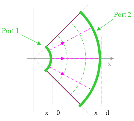
A network on a parabolic coordinate is illustrated. Equipotential lines are in GRN; constant current lines are in MAG. A network laid out on a parabolic coordinates approximates a square root electrical taper.

The coordinates of this system are P and Q where lines of constant P (equipotential) fit:

$\begin{displaymath}P\;=\;\pm\sqrt{\;\sqrt{\,x^2\,+\,y^2\,}\,+\,x\,}\end{displaymath}$

and lines of constant current Q

$\begin{displaymath}Q\;=\;\pm\sqrt{\;\sqrt{\,x^2\,+\,y^2\,}\,-\,x\,}\end{displaymath}$

Referring to the figure, Port 1 is selected such that P = C0; Port 2 is at P = C4. Q is orthogonal to P and the boundary will be Q = ±K

The potential V is determined by applying separation of variables where $V\;=\;F(P)\,G(Q)$ . F and G must satisfy:

$\begin{displaymath}\frac{\,d^2 F\,}{d P^2}\;=\;\left(\,K^2\,-\,s\,\tau\,P^2\,\right)\,F\;=\;0\qquad \qquad\frac{\,d^2 G\,}{d Q^2}\;=\;\left(\,K^2\,+\,s\,\tau\,Q^2\,\right)\,G\;=\;0\end{displaymath}$

To determine r(x) and c(x), the network width along equipotential lines of P must be defined.

x = ½ (D² – Q²) and y = D Q so that:

$\begin{displaymath}x\;=\;\frac{1}{\,2\,}\,\left(\,D^2\,-\,\frac{\,y^2\,}{D^2}\,\right)\end{displaymath}$

The network width along an arc length is found by integrating

$\begin{displaymath}w\;=\;\int_{-D K}^{+D K}\,\sqrt{\,1\,+\,\left(\dfrac{\,d x\,}{d y}\right)^2\;}\;d y\end{displaymath}$

where y = DQ and the network is bounded by ±K

After a bit of tweaking

$\begin{displaymath}w(x)\;=\;K\,\left(\,1\,+\,\sqrt\,2\,x\,+\,k^2\;}\,\right)\,+\,\frac{\,2\,x\,+\,k^2\,}{2}\,\mathit{ln}\,\left[\,\frac{\;K\,+\,\sqrt{\,2\,x\,+\,k^2\;}\,}{\;K\,-\,\sqrt{\,2\,x\,+\,k^2\;}\,}\,\right]\end{displaymath}$

Other methods may be considered but are not discussed here (hasn’t this been enough?)

Design Example: LP Filter

A single stage low-pass filter transfer function is given as

$\begin{displaymath}\frac{\,V_2\,}{V_1}\;=\;\frac{K_o}{\;1\,+\,\dfrac{s}{\,p_o\,}\,}\end{displaymath}$

For a uniformly distributed RC network, the transfer function is modified to

$\begin{displaymath}\frac{\,V_2\,}{V_1}\;=\;\frac{K_o}{\;1\,+\,\dfrac{s}{\,p_o\,}\,}\;N_\varepsilon(s)\end{displaymath}$

where N_ε contains the error poles and zeroes of the network.

Assume the filter is to have a magnitude error of less than 1 dB and a phase error not to exceed 10° from DC to 10 ω_o. N_ε is now constrained to

$0.89\,\le\,| N_\varepsilon (\mathit{j}\omega)|\,\le\,1.12\qquad\qquad \angle N_\varepsilon (\mathit{j}\omega)\,\le\,0.175\,rad\;\;\textnormal{for}\;\;\omega\,\le\,10\,p_o$

At this point, the expression N_ε for has not been determined.

The desired structure is of the form:

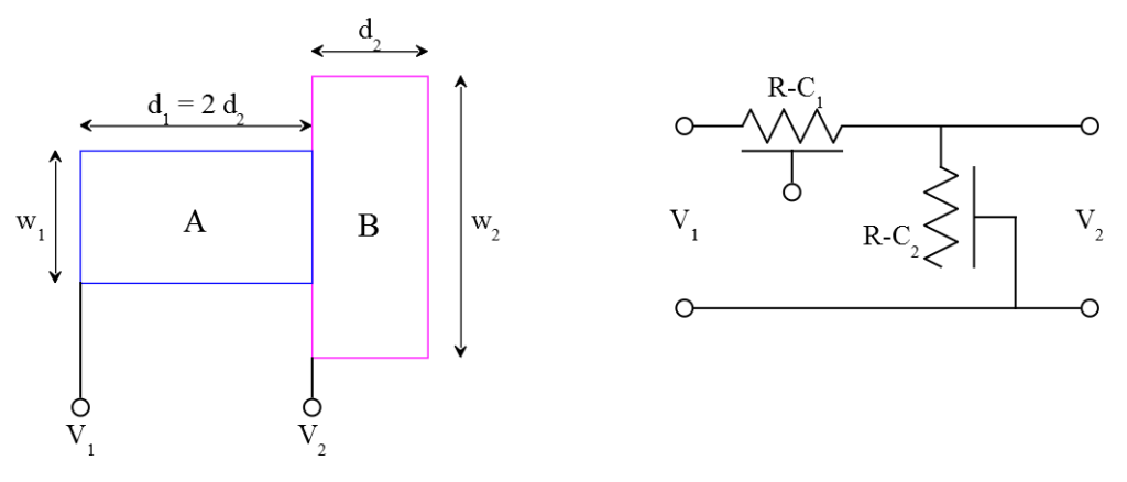
There are two distributed RC networks in which one has twice the dimension d as the other. This network has a transfer function of:

$\begin{displaymath}\frac{\,V_2\,}{V_1}\;=\;\frac{1}{\;\mathit{cosh}\,2\,\Theta_B\,+\,K_1\,(\,\mathit{cosh}\,2\,\Theta_B\,-\,1\,)\,\,}\end{displaymath}$

where $\Theta_B\,=\,\sqrt{\,s\,T_B\,}\,;\;\;T_B\,=\,r_{oB}\,c_{oB}\,;\;\;K_1\,=\,2\,W_B/W_A$ and with poles located at

$\begin{displaymath}p_m\;=\;-\frac{1}{\,4\,T\,}\,\left[\,\eta\,\left(\,\mathit{cos}^{-1}\,\frac{K_1\:}{\,1\,+\,K_1\,}\,\right)\,\pm\,2\,m\,\pi\,\right]^2\end{displaymath}$

The secondary poles are located in pairs at approximately $p_{n_{1,2}}\;=\;\dfrac{\,(\,n\,\pi\,)^2\,}{T_B}$

If $w_s\,\gg\,w_1\; ,\,K_1$ is large and $k\,=\,\mathit{cos}^{-1}\,\dfrac{K_1}{\,1\,+\,K_1\;}\;\ll\;1$

(if K = 10, then k = 0.43; if K = 100, then k = 0.14)

If k << 1, N_ε is approximately

$\begin{displaymath}N_\varepsilon\;\approx\;\prod_{n=1}^\infty\,\left[\,\dfrac{1}{\,1\,+\,\dfrac{s\,T_B}{\,(\,n\,\pi\,)^2\;}\,}\,\right]^2\end{displaymath}$

Expanding the magnitude of this expression:

$\begin{displaymath}\big|\,N_\varepsilon (\mathit{j}\omega)\,\big|^2\;=\;1\,-\,\dfrac{\,(\,\omega\,T_B\,)^2\,}{45}\end{displaymath}$

Applying the network constraints: $\dfrac{\,(\,\omega\,T_B\,)^2\,}{45}\;<\;0.12$ and $\omega \,<\,10\,p_o$

giving $\big|p_o\big|\;<\;\frac{1}{\,T_B\,}\,\sqrt{\,\dfrac{\,0.45\times 0.12\,}{100}\,}\;<\;\frac{\,0.232\,}{T_B}$

With the 2nd dominant pole located at $p_1\,=\,-\pi^2/T_B$

$\big|p_o\big|\;<\;\dfrac{\,0.232\,}{\pi^2}\,\big| p_1 \big| \;<\; \dfrac{\,\big| p_1 \big| \,}{T_B}$

The phase of the error function N_ε is $\angle N_\varepsilon (\mathit{j}\omega)\;\approx\;-2\,\sum_{n=1}^\infty\,\mathit{tan}^{-1}\,\frac{\,\omega\, T_B\,}{\,(\,n\,\pi\,)^2\,}$

If $\omega\;<\;\dfrac{\,(\,n\,\pi\,)^2\,}{T_B\,}$ , the tan^-1 coefficient may be replaced with its angle such that

$\sum_{n=1}^\infty\,\dfrac{1}{\,n^2\,}\;\Rightarrow\;\dfrac{\,\pi^2\,}{6}\qquad\textnormal{and}\qquad \angle N_\varepsilon (\mathit{j}\omega)\;\approx\;-\dfrac{\,\omega\,T_B\,}{3}\;=\;\dfrac{\,\omega\,\pi^2\,}{\,3\,p_1\,}$

At $\omega_o\;=\;10\,p_o$

$\begin{displaymath}0.175\;=\;\frac{\,10\,\pi^2\,p_o\,}{3\,p_1} \;\;\Rightarrpw\;\;p_o\;=\;\dfrac{\,0.525\,p_1\,}{10\,\pi^2}\;=\;\frac{p_1}{\,188\,}\end{displaymath}$

From the magnitude requirements, the 1^st pole must be 43 times further from the origin than p_o. The phase restriction requires that p₁ be 188 times further than p_o

Solving for K

$\begin{displaymath}\mathit{cos}^{-1}\,\dfrac{K_1}{\,1\,+\,K_1\,}\;\le\;\dfrac{2\,\pi}{\,\sqrt{\,188\,}\,}\;=\;0.458\;\;\rightarrow\;\;K_1\,=\,\frac{\,2\,w_B\,}{w_A}\;=\;\frac{\mathit{cos}\,0.458}{\,1\,-\,\mathit{cos}\,0.458\,}\;\;\Rightarrow\;\;K_1\,=\,8.5\end{displaymath}$