Wheatstone Bridge – Dave McGlone

The Wheatstone Bridge is a simple circuit capable of making very accurate measurements. The basic network was actually proposed in the 1830s by Samuel Christie but named after Charles Wheatstone who publicly presented it – as Christie’s work – in 1843. It remains the basis for many transducer interface networks to this day.

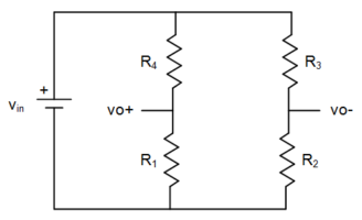
$\begin{displaymath}V_{out} \; = \; v_o^+ \, - \, v_o^- \; &= \; V_{in} \, \left( \, \frac{R_1}{ \, R_1 \, + \, R_4 \, } \, \right) \; - \; V_{in} \, \left( \, \frac{R_2}{ \, R_2 \, + \, R_3 \, } \, \right)\end{displaymath}$

$\begin{displaymath}V_{out} \; = \; V_{in} \, \left[ \, \frac{ \frac{R_1}{\, R_4 \, } \, - \, \frac{R_2}{\, R_3 \, } }{\, \left( \, 1 \, + \, \frac{R_1}{\, R_4 \, } \, \right) \, \left( \, 1 \, + \, \frac{R_2}{\, R_3 \, } \, \right) \, } \, } \, \right]\end{displaymath}$

The system is in balance when V_out = 0 … or when (R₁/R₄) = (R₂/R₃). Note that this is a ratiometric comparison. Note also it is non-linear.

Consider the situation where R₁ = R₂ = R₃ = R₁ = R but allow R₁ to vary by ΔR due to some influence … perhaps temperature, strain, or some such.

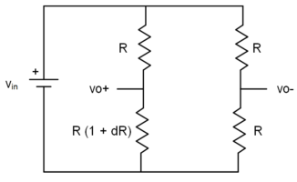
The bridge expression may now be expressed:

$\begin{displaymath}V_{out} \; = \; V_{in} \, \left[ \, \frac{R_1 \, (1 \, + \, \Delta R)}{ \, R_1 \, (1 \, + \, \Delta R) \, + \, R_4 \, } \; - \; V_{in} \, \frac{R_2}{ \, R_2 \, + \, R_3 \, } \, \right]\end{displaymath}$

$\begin{displaymath}V_{out} \; = \; V_{in} \, \frac{\Delta R}{ \, 4 \, + \, 2 \, \Delta R \, }\end{displaymath}$

The absolute value of R is not part of the expression.

The sensitivity of function y to a change in parameter x of that function is defined:

$\begin{displaymath}S_x^y \; \equiv \; \frac{ \, \partial y / y \,}{ \, \partial x / x \,} \; = \; \frac{x}{\, y \,} \, \frac{ \, \partial y \,}{\partial x}\end{displaymath}$

which gives the sensitivity of the output to a change in R₁ of:

$\begin{displaymath}S_{\Delta R_1}^{V_{out}} \; = \; \frac{2}{ \, 2 \, + \, \Delta R_1 \,}\end{displaymath}$

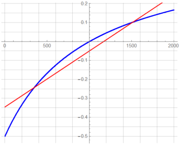
Follows is a plot for $\Delta$ R between -100% and +100% ( R₁ = 0 → +2 for R = 1 ). V_out has the following non-linear response:

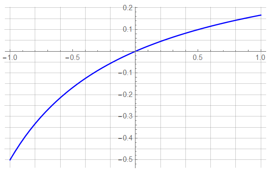
However, if ΔR is small – say no more than ±1%, the response is:

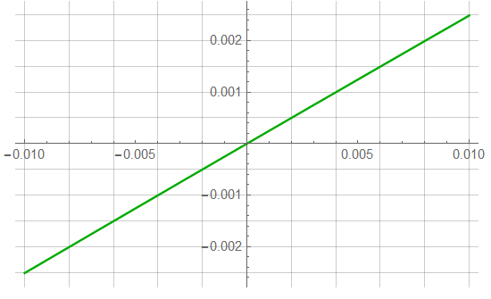
which has an $\mathbb{R}^2$ value of 0.999993. A fairly linear response …

A 10% change has an $\mathbb{R}^2$ value of 0.999332; a 30% change has value of 0.993929.

A plot comparing the output vs. a linear regression at 10% variation in ΔR:

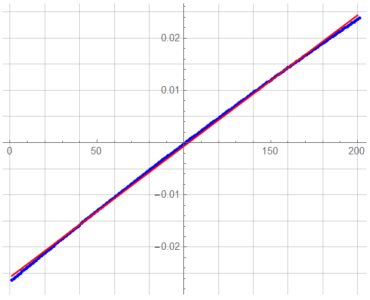
The BLU line is the output for ΔR = ±10%; the RED line is the result of the linear regression.

This is often sufficient for many measurements but some transducer variations may exceed the range where a linear assumption remains valid.

The value at ΔR = 0 is -0.0257 … a perhaps unacceptable error of 2.6%. This is the same magnitude error (to 2 places) at the extremities as well. The true response is non-linear; a simple offset adjustment is not suitable.

It would be a stretch to assume a “linear” response for a variation of ΔR = ±100% … even if the $\mathbb{R}^2$ value is 0.923227 – which suggests that an $\mathbb{R}^2$ value of even 0.92 is subjectively not very good. Of course, “accurate” is relative.

A means of linearizing the output over a wide range of ΔR is possible though.

Consider the following topology:

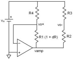
The opamp is configured such that vo+ is forced to GND through the virtual GND connection at the inverting input (recalling that the inverting input is isolated from but at the same potential as the non-inverting input). Since vo+ is at GND potential, the current through R4 is V_in/R4 … and the same current flows through R1 regardless of the value of dR.

This forces the voltage drop across R1 to be:

$\begin{displaymath}V_{R_1} \; = \; I_{R_4} \, R_1 \, \right) \; = \; \frac{\, V_{in} \, }{R_4} \, R_1 \; = \; V_{in} \, \frac{R_1}{ \, R_4 \, }\end{displaymath}$

The opamp will force the voltage at the opamp output to be:

$\begin{displaymath}V_{amp} \; = \; vo^+ \, - \, V_{R_1} \; = \; 0 \, - \, V_{in} \, \frac{R_1}{ \, R_4 \, }\end{displaymath}$

The current through the 2nd branch (R3/R2) is:

$\begin{displaymath}I_2 \; = \; \frac{ \, V_{in} \, - \, V_{amp} \, }{R_2 \, + \, R_3} \; = \; \frac{ \, V_{in} \, + \, V_{in} \, \left( \, \frac{R_1}{ \, R_4 \, } \, \right) \, }{R_2 \, + \, R_3} \; = \; V_{in} \, \frac{ \, 1 \, + \, \frac{R_1}{\, R_4 \, } \, }{R_2 \, + \, R_3}\end{displaymath}$

So that vo^– may be determined from:

$\begin{displaymath}vo^- \; = \; V_{in} \, - \, I_2 \, R_3 \; = \; \frac{ \, V_{in} \, - \, V_{amp} \, }{R_2 \, + \, R_3} \, R_3\end{displaymath}$

and

$\begin{displaymath}V_{out} \; = \; V_{in} \, \frac{\, R_3 \, }{R_2 \, + \, R_3} \, \left[ \, 1 \, + \, \frac{\, R_1 \, (1 \, + \, \Delta R ) \, }{R_4} \, \right]\end{displaymath}$

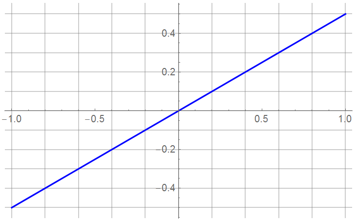
With an ideal opamp configured as previously shown and all resistors of equal value:

$\begin{displaymath}V_{out} \; = \; vo^+ \; - \; vo^- \; = \; V_{in} \, 0.5 \, \Delta R\end{displaymath}$

which, when plotted for $\Delta R \, = \, \pm \, 100\%$ , has a linear response of:

Keeping in mind the ratiometric balance, consider that R3 and R4 are scaled values of R1 and R2 such that R3 = R4 = x R. The output voltage is now calculated as:

$\begin{displaymath}V_{out} \; = \; V_{in} \, \frac{dR}{\, 1 \, + \, x \, }\end{displaymath}$

The response is still linear as long as value $x$ is a constant.

Possible error sources include quality of $V_{in}$ , quality of resistor matching, and opamp characteristics … but all in all, a linearization of a Wheatstone bridge over a wide variance of single-element change.

That’s good for now.

Leave a Comment Cancel Reply