Once concept I find ignored quite a bit – including myself among the guilty – are the assumptions for “small-signal” analysis.
As taught in introductory classes, small-signal analysis occurs over an infinitesimal increment about some fixed operation point (which used to be known as the “Q” point – for “quiescent”. Is it still? I haven’t heard the term in years).
The incremental change required dealing with derivatives but in the incremental model, the derivative became a linear change “ “. While this is correct given the basic assumptions, it seems we get in the habit of thinking that “linear systems” are indeed always linear. Even resistors are not necessarily linear over temperature if a 2nd-order tempco term is significant (and included in the model).
How far not linear? It depends on the specific situation.
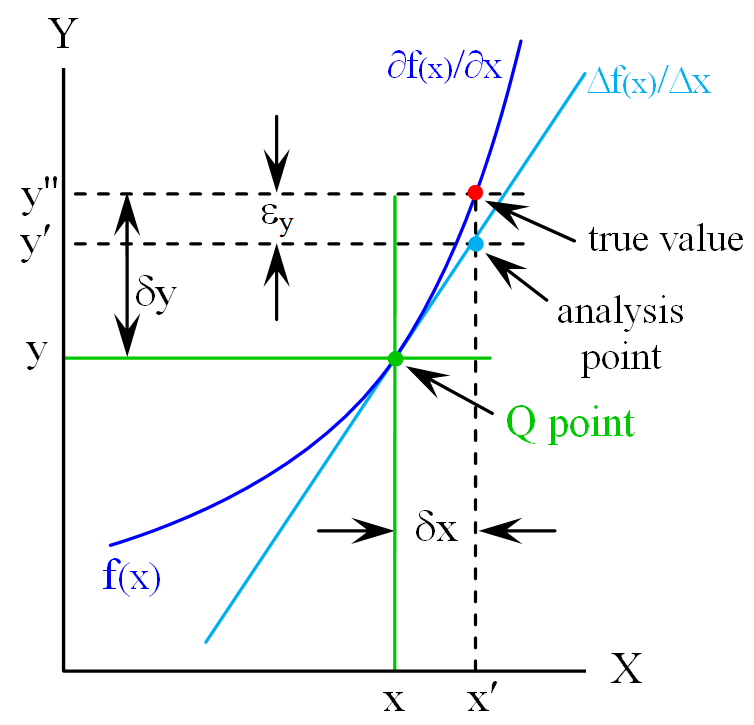
Referring to the figure, the network has function f(x) indicated in BLU with response y indicated as operating point Q for condition x marked in GRN. A small-signal analysis assumes linearity in the near-vicinity of Q (CYN). With a change of condition x to x’, the expected value of the output f(x’) is predicted to be y’. However, the linearity assumption has failed to the point where the true value of f(x’) is y”.
Is this significant? Not if error  is within acceptable performance limits.
Consider a simple MOS amplifier. The Q-point might represent the bias point with no input. The gain is determined by small-signal analysis: the output response is determined by assuming an incremental linear input stimulus. This small-signal assumption is often applied to the entire operating range – which granted, is small itself with supply voltage of 1.8 or 3.3V. For MOSFETs in particular, this is equivalent to applying the square-law to the relationship between gate voltage and drain current over the entire operating range – but with smaller geometries, the square-law rarely applies for more than a small segment of the operating range – and with small geometries, the square-law itself may not apply.
The small-signal assumption is properly applied to ideally infinitesimally small variations about the operating point. In practice, this “infinitesimally small variation” should be limited to 1 or 2% of the operating range – 5% on the outside. For a 3.3V supply, this suggests applicability over only a few 10s of mV.
Computers only calculate functions given to them. If the underlying model is flawed, so will be the result. Trouble is, one can get by in the vast majority of situations. But for precise work, close enough isn’t good enough.
While perfection is the enemy of good enough (and schedule and budget), “good enough” is also a means of turning the desired square into a circle from excessive cutting of corners.
![]()