_ADC New 9 Timing Uncertainty

When “errors” are considered, they usually relate to magnitude – and often to noise voltage or current. However, clocked systems such as the sampling process may be susceptible to timing variations which lead to measurement errors as well. I’ll discuss the issue based on sampling for ADCs, but the concepts may apply to any timed system.

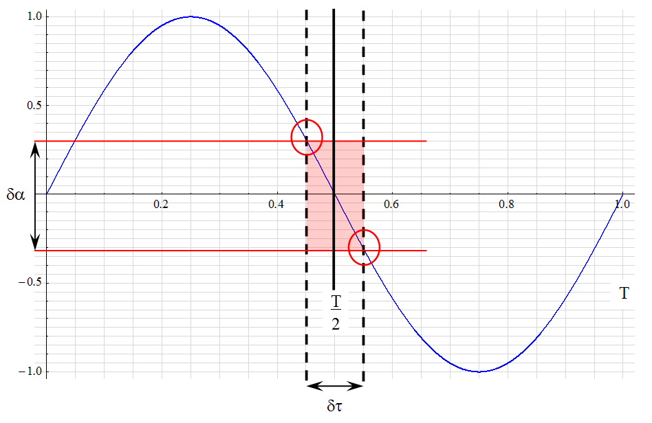
Consider a sampling process with timing uncertainty $\delta \tau$ as shown in the figure below. This uncertainty causes an amplitude uncertainty $\delta \alpha$ in the ideal BLU signal within the limits bounded by RED.

This effect is known as aperture jitter which manifests itself as an increase in quantization noise.

The slew rate of the signal at the ideal Nyquist sample point of T/2 is expressed as the time derivative of the signal at that point:

$\begin{displaymath} \text{SR} \; = \; \frac{d}{\,dt \,} \, V_p \, sin(\, \pi \, f_s \, t) \; = \; \pi \, f_s \, V_p \end{displaymath}$

This expression can relate the signal amplitude uncertainty to the time uncertainty as:

$\begin{displaymath} \frac{ \, \Delta V_s \, }{\Delta T_s} \; = \; \pi \, f_s \, V_p \; \; \Rightarrow \; \; \Delta V_s \; = \;\pi \, f_s \, V_p \, \Delta T_s \end{displaymath}$

If the maximum amplitude error is limited to ½ LSB, the maximum time uncertainty is limited to:

$\begin{displaymath} \Delta T_s \; \leq \; \frac{1}{ \, 2^N \, \pi \, f_s \, } \end{displaymath}$

The average value of the sample point is found by integrating the sample time probability over time:

$\begin{displaymath} \tau_{avg} \; = \; \int\limits_{-\infty}^{+\infty} \rho (t) \, t \; dt \end{displaymath}$

If the actual sample point can occur with equal likelihood at any point within the bounds of $\delta \tau$ , it is said to have a uniform probability distribution (aka, “rectangular”, or “boxcar”).

The average value is then found to be:

$\begin{displaymath} \tau_{avg} \; = \; \int\limits_{-\delta \tau /2}^{+\delta \tau /2} \rho (t) \, t \; dt \; = \; \int\limits_{-\delta \tau /2}^{+\delta \tau /2} \frac{1}{\, \delta \tau \,} \, t \; dt \; = \; 0 \end{displaymath}$

The variance $^\textbf{\large 1}$ of such a function is the average of the square of the deviation from the average value:

$\begin{displaymath} \sigma^2 \; = \; \int\limits_{-\delta \tau /2}^{+\delta \tau /2} \rho (t) \, t^2 \; dt \; = \; \frac{ \, \delta \tau^2 \, }{12} \end{displaymath}$

from which the standard deviation is determined:

$\begin{displaymath} \sigma \; = \; \frac{ \, \delta \tau \, }{\sqrt{12}} \end{displaymath}$

As an example, assume a 10 MHz sample rate on a 12-bit converter. The maximum allowable clock jitter would be:

$\begin{displaymath} \Delta T_s \; < \; \frac{1}{ \, 2^{12} \, \pi \, (10\text{e6}) \, } \; = \; 7.8 \; ps \end{displaymath}$

In terms of timing stability:

$\begin{displaymath} \Delta T_{s,ppm} \; < \; \frac{\, 7.8\text{e-12} \,}{\, 100\text{e-9} \,} \; = \; 7770 \; ppm \end{displaymath}$

This calculation assumes sampling at the Nyquist frequency.

By expressing the time uncertainty in terms of signal frequency rather than sample frequency …

$\begin{displaymath} \Delta T_s \; < \; \frac{1}{ \, 2^N \, 2 \, \pi \, f_{in} \, } \end{displaymath}$

If the signal frequency is limited to ¼ fs, then:

$\begin{displaymath} \Delta T_s \; \leq \; \frac{1}{ \, 2^{12} \, \pi \, \frac{\, 10\text{e6} \,}{2} \, } \; = \; 15 \, 500 \; ppm \end{displaymath}$

The previous analyses were based on a uniform distribution of time uncertainty within fixed limits. However, it is possible the probability distribution will be of the form of a normal or Gaussian distribution $^\textbf{\large 2}$ such that:

$\begin{displaymath} \rho (t) \; = \; \frac{1}{ \, \sigma \, \sqrt{ \, 2 \, pi \, } \, } \, exp \left( \, \frac{t^2}{\, 2 \, \sigma^2 \, } \, \right) \end{displaymath}$

From which the variance may be estimated:

$\begin{displaymath} \sigma^2 \; = \; \frac{\, \delta \tau^2 \,}{ 36 } \; \Rightarrow \; \sigma \; = \; \frac{\, \delta \tau \,}{6} \end{displaymath}$

where 6 $\sigma$ ≈ $\delta \tau$ .

At any given time, the error of the sampled voltage is:

$\begin{displaymath} \Delta V_s \; = \; \Delta T_s \, V_p \, 2 \, \pi \, f_{in} \; cos(2 \, \pi \, f_{in} \, t) \end{displaymath}$

And at some discrete time step:

$\begin{displaymath} \Delta V_s(nT) \; = \; \Delta T_s(nT) \, V_p \, 2 \, \pi \, f_{in} \; cos(2 \, \pi \, f_{in} \, n \, T) \end{displaymath}$

This function has aliased terms which require filtering for frequencies above fs/2.

The example system signal has peak value of 0.5 and a sample frequency of 100 MHz. If it is assumed the signal frequency is ½ the Nyquist frequency (or ¼ the sample frequency) and the maximum clock jitter is 100 ps, then the average power of the error signal is found as:

$\begin{displaymath} \begin{align} P_{avg} \; &= \; \sigma^2 \, \frac{ \, \left( \, V_p \, 2 \, \pi \, f_{in} \, \right)^2 \,}{2} \; = \; \frac{\, \delta \tau^2 \, }{36} \, \frac{\, \left( \, V_p \, 2 \, \pi \, f_{in} \, \right)^2 \, }{2} \\ \\ & = \; \frac{\, (100\text{e-12})^2 \, }{36} \, \frac{\, \left[ \, 0.5 \times 2 \, \pi \, (25\text{e6} \, \right]^2 \, }{2} \; = \; 856.7\text{e-9} \; V^2 \end{align} \end{displaymath}$

The RMS voltage due to clock jitter is 926 μV.

The inherent quantization noise of a 12-bit converter is:

$\begin{displaymath} V_{qe} \; = \; \frac{\text{FSR}}{ \, 2^{12} \, \sqrt{ \, 12 \, } \, } \; = \; 70.5 \; \mu V \qquad \left( \, V_{qe}^2 \; = \; 4.97\text{e-9} \, \right) \end{displaymath}$

The total noise is therefore:

$\begin{displaymath} V_{qe} \; = \; \sqrt{ \, V_{qe}^2 \, + \, V_{jit}^2 \, } \; = \; \sqrt{ \, (70.5\text{e-6})^2 \, + \, (856.7\text{e-9})^2 \, } \; = \; 928 \; \mu V \end{displaymath}$

The jitter noise is considerably greater than the inherent quantization noise. The effect of the jitter is to lower the effective resolution of the ADC:

$\begin{displaymath} \text{SNR} \; = \; \frac{\frac{V_p}{\sqrt{\, 2 \, }}}{\, V_{n,rms} \,} \; \rightarrow \; \frac{\frac{\, 0.5 \,}{\sqrt{\, 2 \, }}}{\, 928\text{e-6}\,} \; = \; 51.62 \; dB \end{displaymath}$

The effective resolution of this 12-bit ADC has been reduced to:

$\begin{displaymath} N_{eff} \; = \; \frac{\, 51.62 \, - \, 1.76 \,}{6.02} \; = \; 8.28 \; \equiv \; 8 \; bits \end{displaymath}$

Consider the situation with a 16-bit ADC.
The inherent quantization noise of a 16-bit converter is:

$\begin{displaymath} V_{qe,16} \; = \; \frac{\text{FSR}}{ \, 2^{16} \, \sqrt{ \, 12 \, } \, } \; = \; 4.40 \; \mu V \qquad \left( \, V_{qe}^2 \; = \; 19.4\text{e-12} \, \right) \end{displaymath}$

The total noise is now:

$\begin{displaymath} V_{qe} \; = \; \sqrt{ \, (4.40\text{e-6})^2 \, + \, (856.7\text{e-9})^2 \, } \; = \; 926 \; \mu V \end{displaymath}$

$\begin{displaymath} \text{SNR} \; = \; \frac{\frac{\, 0.5 \,}{\sqrt{\, 2 \, }}}{\, 926\text{e-6}\,} \; = \; 51.64 \; dB \end{displaymath}$

$\begin{displaymath} N_{eff} \; = \; \frac{\, 51.64 \, - \, 1.76 \,}{6.02} \; = \; 8.28 \; \equiv \; 8 \; bits \end{displaymath}$

The increase in ADC resolution offers no improvement in data precision or accuracy.

Part 9
Part 11

That’s good for now.

$^\textbf{\large 1}$ The variance of a physical signal represents the average power of a signal; the standard deviation represents the RMS value of a signal.

$^\textbf{\large 2}$ The specific distribution of time variance has much to do with the nature of the timing source. A digitally-derived clock may have a uniform distribution; a quartz oscillator may be Gaussian in nature. As they say: YMMV.