To this point, frequency-domain issues have been discussed. Additional information may be taken from field measurements made in the time domain. By assuming a linear system, the analysis is based upon:
Output(s) = Input(s) × System(s) ⇔ Output(t) = Input(t) * System(t)
where multiplication in the Laplace domain is equivalent to convolution in the time domain.
The conversion between domains is accomplished with the Laplace Transform:
![\begin{displaymath} \mathcal{L}\left[\, f(t) \, \right] \; = \, F(s) \end{displaymath}](https://davemcglone.com/wp-content/ql-cache/quicklatex.com-417bfc8d8dc7ff16e9ecc21a71a42d5c_l3.png "Rendered by QuickLaTeX.com")
A system function (the earth and any anomalies) may be determined if the input stimulus is adequately characterized and the output response is adequately measured. This basic rationalization for subsurface interpretation assumes the source signal is adequately known. If sufficient measurements are made to characterize the response, an interpretation of the subsurface structure may be made. However, “adequate” is a nebulous term …
A measured field is a composite of all fields present at the time of observation. Neglecting any external sources, the measured field is the sum of the primary field generated by the source and the secondary fields generated by conductive zones within the host material.
The secondary field contains the desired information; a transient, or time-domain, exploration is conducted by turning the primary field off and measuring the decay of the secondary field. A frequency-domain exploration measures the field at particular frequencies with an active transmitter. The anomalies are inferred by the distortion characteristics of the received data.
While frequency-domain measurements are made with a quasi-static source, time-domain measurements are made in the presence of a transient source field. Typically, these measurements occur immediately after the source is turned off. The bandwidth of the receiver is a critical parameter in determining the effectiveness of a time-domain exploration. A receiver with sufficient bandwidth can make both types of measurements during a single measurement sequence.
A possible transmitter source stimulus may be expressed in the Laplace domain as:
![\begin{displaymath} M(s) \; = \; M_o \, \left[ \, \frac{1}{s} \, + \, \frac{1}{\, t_r \, s^2 \,} \, \left( \, \mathbb{e}^{-\, t_r \, s} \, - \, 1 \,\right) \, \right] \end{displaymath}](https://davemcglone.com/wp-content/ql-cache/quicklatex.com-0db65d55982a9030e8a52c29eb73dd84_l3.png "Rendered by QuickLaTeX.com")
Based on the frequency domain expressions, the time domain magnetic field response on the surface may be expressed with:
![\begin{displaymath} \begin{align} B_z(t) \; = \; &\frac{\, M_o \, \mu_o \,}{2 \, \pi \, \rho^3} \, \left[ \, \frac{\, 9 \, t \,}{\alpha^2} \, + \, \frac{\alpha}{\, \sqrt{\, \pi \, t \, } \, } \, \mathbb{e}^{-\phi^2} \, + \, \left( \, \frac{\, 36 \, t \,}{\alpha^2} \, + \, 4 \, - \, \jmath \, \frac{ \, 18 \, \sqrt{\, t \, }}{\alpha} \, \right) \, \text{erfc} \, \phi \right. \\ \\ \left. &+ \; \delta \left\{\, \frac{9 \, t^2}{\, 2 \, t_r \, \alpha^2 \,} \, + \, \left[ \, \frac{36 \, t^2}{\, t_r \, \alpha^2 \, } \, - \, \frac{\, 16 \, t \,}{t_r} , + \, \jmath, \left( \, \frac{\, 2\, \alpha \, \sqrt{\, t \, } \, }{t_r} \, - \, \frac{\, 72 \, \sqrt{\, t^3 \, } \, }{t_r \, \alpha} \, \right) \, \right] \, \text{erfc} \, \phi \right] \end{align} \end{displaymath}](https://davemcglone.com/wp-content/ql-cache/quicklatex.com-77645dfcefa7b3c673fc21337b9e5f97_l3.png "Rendered by QuickLaTeX.com")
Using the target of Part 4, the following secondary field time response at the surface to an ellipsoidal target is estimated. The first plot is a map of the Bz “measurement” over the target area. This is a small target (10″ x 10 ft) located 30 ft away from the dipole and buried 10 ft deep. The magnetic dipole magnitude is 1000 A m^2; the relative conductivity ratio is 0.001/0.0002 = 5. The object is centered about the y-axis, the scale “X” is a measure off that axis.
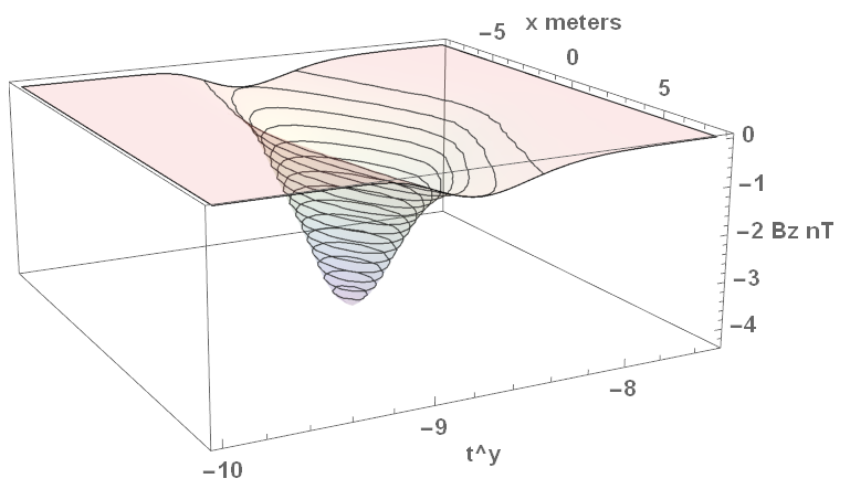
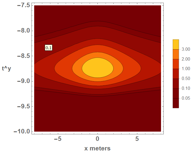
The following is a contour map of the above. Contour colours run dark to light with magnitude; the lines are as labeled on the legend. The y-axis is based on a step function of the source. The labels are the exponent of the time response – peak magnitude of about 4.3 nT occurs at the center of the conductive body approximately 2 ns ( ) after the source is switched on. An “early time” situation …
So far, so good, and …
That’s good for now.
![]()