Filtering – Part 6 – Dave McGlone

I left the last section with a moderately complex continuous-time waveform segment and a demonstration that a mathematically perfect signal with mathematically perfect Nyquist sampling indicates no frequency content. I know – you know – that in the engineering world, mathematically perfect doesn’t exist; “0” is very small, “∞” is very large – but both are finite numbers.

My primary goal in these discussions has been to discuss the effects of filtering on a measurement signal that is to be digitized. The choice of filter type, order, and sampling parameters can greatly affect the “garbage in” portion of GIGO; hopefully, I’ll show some of the undesirable effects that may not be directly obvious at first – and certainly not later when the data has been quantized and undergoing interpretation.

The filters have been developed in the frequency-domain but signals are measured in the time-domain. The effects of the filters was most apparent in phase lag – group delay – but amplitude changes also contribute to signal distortion.

Recall the basic signal chain map presented in Part 1:

At this point of the discussion, we are at the ADC input. The ideal signal has been converted to an electronic signal – voltage or current – and filtered; it is now ready to be quantized … quite often with a converter output consisting of a sequence of digital words of N-bit width. The signals are perfect, the filters are perfect, and there is no noise or component uncertainty added.

I’ll use 4th-order filters: the frequency-normalized Butterworth and the delay-normalized Bessel.

As a reminder, the Butterworth function may be found from:

$\begin{displaymath} \begin{align} \sum_{k=1}^n \; exp \left[\, \em j \, \pi \, \frac{2 \, k \,+ \, n \, - \, 1 \, }{2 \, n \, } \right] \end{align} \end{displaymath}$

and the Bessel:

$\begin{displaymath} \begin{align} \sum_{k=0}^n \; \frac{s^k \, ( \, 2 \, n \, - \, k \, ) \, ! \, }{2^{n \, - \, k \, } \, k\,! \,( \, n \, - \, k \, ) \, !} \end{align} \end{displaymath}$

From which, the 4th-order filter functions are:

$\begin{displaymath} \begin{align} T_{bw}(s) \; &= \; \frac{1}{1 \, + \, 2.61313 \, s \, + \, 3.41421 \, s^2 \, + \, 2.61313 \, s^3 \, + \, s^4 \, } \quad &\Rightarrow \quad T_{bw,mag}(\omega) \; &= \; \frac{1}{\, \sqrt{\, \left(\, 2.61313 \, \omega \, - \, 2.61313 \, \omega^3 \, \right)^2 \, + \, \left( \, 1 \, - \, 3.41421 \, \omega^2 \, + \, \omega^4 \right)^2 \, }} \\ \\ T_{be}(s) \; &= \; \frac{105}{105 \, + \, 105 \, s \, + \, 45 \, s^2 \, + \, 10 \, s^3 \, + \, s^4 \, } \quad &\Rightarrow \quad T_{be,mag}(\omega) \; &= \; \frac{105}{\, \sqrt{\, 25 \, \omega^2 \, \left(\, 21 \, - \, 2 \, \omega^2 \, \right)^2 \, + \, \left( \, 105 \, - \, 45 \, \omega^2 \, + \, \omega^4 \right)^2 \, }} \end{align} \end{displaymath}$

The phase and group delay equations get “messy”; the group delay expressions are:

$\begin{displaymath} \begin{align} \tau_{bw}(\omega))\: &= \: \dfrac{\frac{\, 2.61313 \: - 7.83938 \, \omega^2 \,}{\, 1 \, - \, 3.41421 \, \omega^2 \, + \, \omega^4 \,} \: - \: \frac{\left( \, 2.61313 \, \omega \: - 2.61313 \, \omega^3 \, \right) \; \left( \, 4 \, \omega^3 \, - \, 6.82843 \, \omega \, \right) }{\, \left( 1 \, - \, 3.41421 \, \omega^2 \, + \, \omega^4 \, \right)^2 \, }}{\, 1 \, + \, \frac{\left( \, 2.61313 \, \omega \: - 2.61313 \, \omega^3 \, \right)^2 }{\, \left( 1 \, - \, 3.41421 \, \omega^2 \, + \, \omega^4 \, \right)^2 \, }} \\ \\ \tau_{be}(\omega)\: &= \: \dfrac{\frac{5 \, \left( \, 21 \, - \, 2 \, \omega^2 \, \right)}{105 \, - \, 45 \, \omega^2 \, + \, \omega^4} \, \left[ \, 1 \, - \, \frac{\omega \, \left( \, 4 \, \omega^3 \, - \, 90 \, \omega \, \right)}{105 \, - \, 45 \, \omega^2 \, + \, \omega^4} \, \right] \, - \, \frac{20 \, \omega^2}{105 \, - \, 45 \, \omega^2 \, + \, \omega^4}}{1 \, + \, \frac{25 \, \omega^2 \, \left( \, 21 \, - \, 2 \, \omega^2 \, \right)^2}{\, \left( \, 105 \, - \, 45 \, \omega^2 \, + \, \omega^4 \, \right)^2} \, } \end{align} \end{displaymath}$

And after all this background, I get to the point of this portion of the discussion: the ideal quantization.

While the physical phenomena to be measured is analog in nature, it is stored and processed in digital form. Ignoring the limiting effects of a practical ADC, I’ll assume impulse sampling – the sample point is the instantaneous value of the time function without quantization error (the finite magnitude range of each bit). The time function is sampled every Δt interval so that a sequence of representative values is obtained.

The number of elements is the length of time the measurement is made divided by Δt: if a 1Hz signal is sampled such that Δt = 1/10 sec and information is collected over 1 sec of time, the data sequence will be:

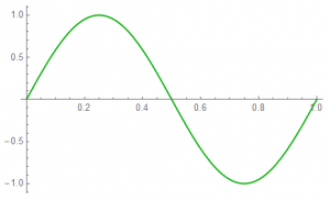
$\begin{displaymath} data[n] = \left[ \left( 0, 0 \right), \left( \, \dfrac{1 \, \pi}{5}, \, 0.587785 \, \right), \left( \dfrac{2 \,\pi}{5}, 0.951057\right), \left( \dfrac{3 \,\pi}{5}, 0.951057 \right), \left( \dfrac{4 \,\pi}{5}, 0.587785 \right), \left( \,\pi, \, 0 \right), \left( \dfrac{6 \,\pi}{5}, -0.587785 \right), \left( \dfrac{7 \,\pi}{5}, -0.951057 \right), \left( \dfrac{8 \,\pi}{5}, -0.951057 \right), \left( \dfrac{9 \,\pi}{5}, -0.587785 \right), \left( 2 \pi, \, 0 \right)\, \right] \end{displaymath}$

The continuous-time waveform appears as:

The sampled time sequence of data is represented by the RED dots; the BLU represents the continuous-time source.

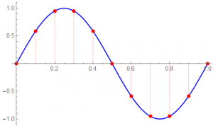
The last point is not used in the single-cycle analysis; it belongs to the next cycle.

For analysis, I use Mathematica as a simulation program. Mathematica uses the following definition for the Fourier calculations:
The Discrete Fourier Transform $F_s$ of a sampled sequence X of length N is:

$\begin{displaymath} \dfrac{1}{\, \sqrt{\, N \, } }\; \sum_{n \, = \, 1}^N \left( \, X_n \, exp\left[\, 2 \, \pi \, (n-1)(s-1)/N \right] \, \right) \end{displaymath}$

The first term is the zero-th frequency; N need not be a power of 2.

The result of such a calculation gives information of magnitude and phase – a sampled data version of a Bode Plot:

At 10 samples over 1 cycle, the magnitude result:

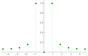
Looking at the positive half-spectrum – the plot of most interest:

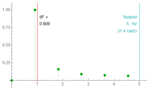
The RED line indicates the exact frequency … sampling at 10x the signal frequency is not sufficient to accurately determine the frequency – the analysis indicates f1 = 0.91 Hz rather than the actual 1.0 Hz. Significant? Could be … depends on the project goals.

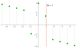
The phase spectrum:

Just how much sampling is necessary? Depends on the project but I want to look at some examples. I’ll use one cycle of a 1 Hz signal – $sin[\, 2 \, \pi \, t \,]$ – as the signal and vary the sample frequency using prime numbers. Lots of plots here …

Start with the highest frequency and work down. The exact frequency on the spectrum charts is marked with RED line; all magnitudes are normalized to 1. I’ll show four plots for each sample rate: 1) continuous time with sample points indicated; 2) the full spectrum; 3) the positive half of the spectrum; 4) the phase spectrum.

Note that these plots present the sample frequency as samples per cycle. For example, the first plot has the sample frequency 2003x the signal frequency – a 2 GHz sample rate for a 1 MHz signal. The plots of greatest interest for amplitude measurements would be the positive half-spectrum but the amplitude response is normalized for these plots.

Sample Rate: 2003

With 2003 sample points, the plot almost appears continuous at this scale.

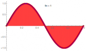
It’s difficult to discern the two frequency spikes at this scale.

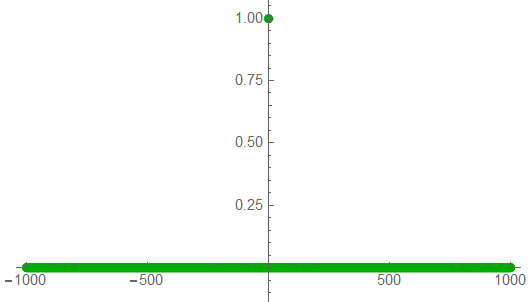
Taking a closer look:

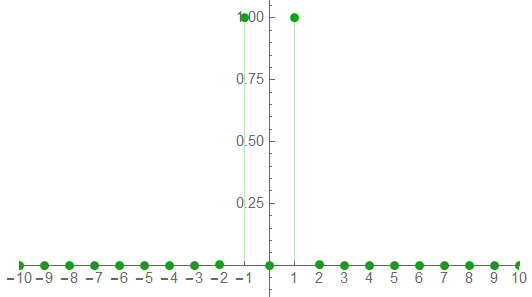
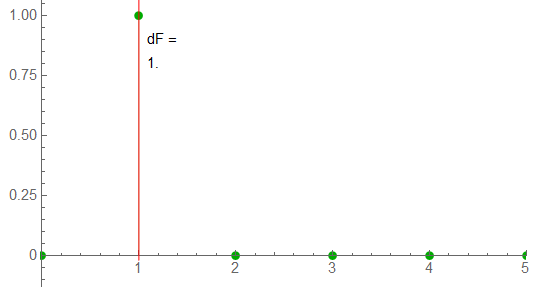
As expected, the indicated frequency is 1 with no apparent energy spill-over.

The full phase response …

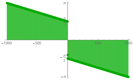
… and a truncated version:

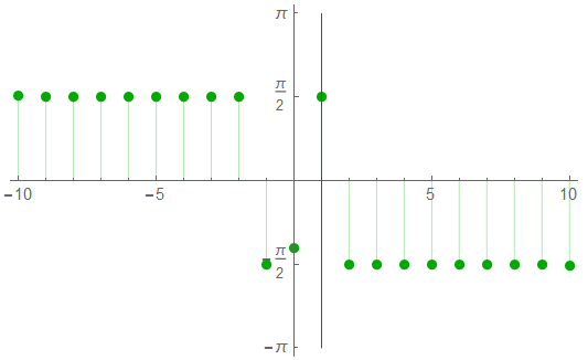
The half-spectrum indicates a frequency increment of 0.99950 … or 1.000 to 3 decimal places:

In many situations, this sample rate would be over-kill.

Sample Rate: 211

The sample rate has been lowered by about a factor of 10 (but again a prime number). Many, many samples per cycle, but individually distinguishable by eye at this scale.

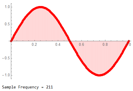
The full spectrum on a truncated plot …

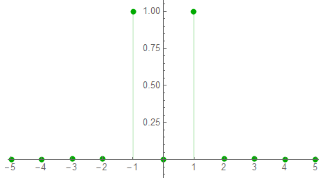
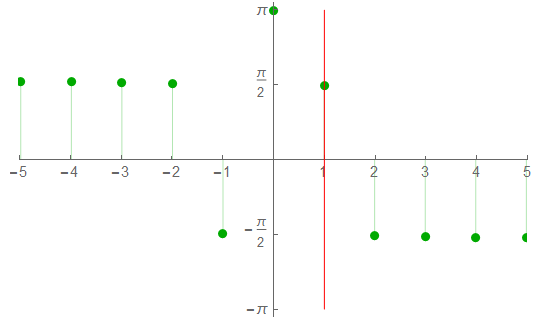
The phase spectrum on a truncated plot.

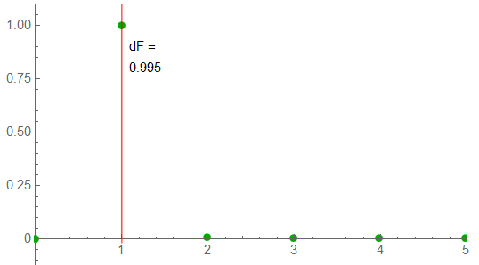
The positive frequency spectrum has a frequency increment is off the ideal by 5 mHz – too small to detect at this scale.

This sample rate could also be considered over-kill in many situations.

Sample Rate: 23

When I was first working on high-precision circuitry early in my career, the rule-of-thumb for an initial sample rate was 20 to 50 times the highest signal frequency. This represents the lower end of that scale (while the previous example was 4x the higher end of that rule)

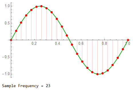
The spectrum begins to indicate some energy spill-over. Whether this is critical or not depends on project goals … but could indicate a need to bump the sample frequency up a touch.

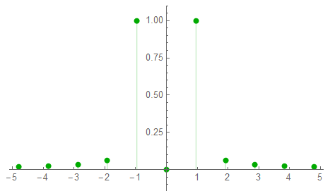
The half-phase plot:

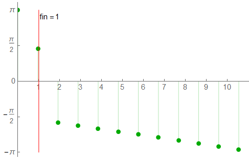
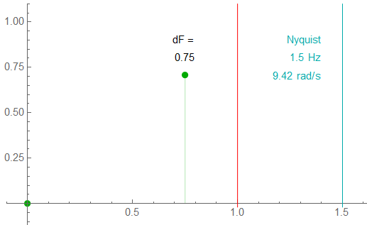
The positive half-spectrum plot distinctly shows a bit of offset between indicated frequency and the actual frequency. The frequency step is about 5% off the nominal frequency. Energy spreading is becoming apparent.

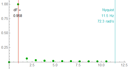
Sample Rate: 3

Although above the Nyquist limit, a sample rate of 3x the signal frequency is only sufficient for gross measurements.

The full spectrum:

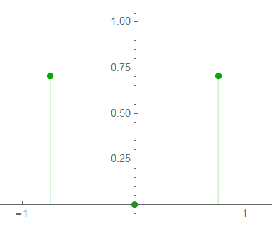
The phase plot shows the frequency offset:

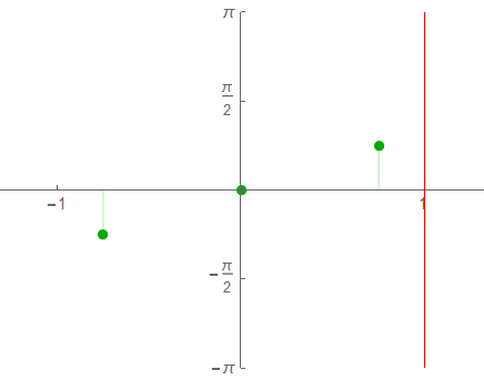
The positive spectrum shows the energy split between frequency “bins”. The resolution is 33%; it would be difficult to measure amplitude if the nominal frequency was unknown … unless the goal is simply to determine whether significant energy exists in this range.

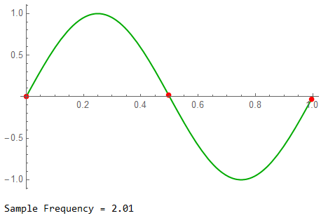
Sample Rate: 2.01

The Nyquist limit. The use of 2.01 instead of 2.0 allows a non-zero response.

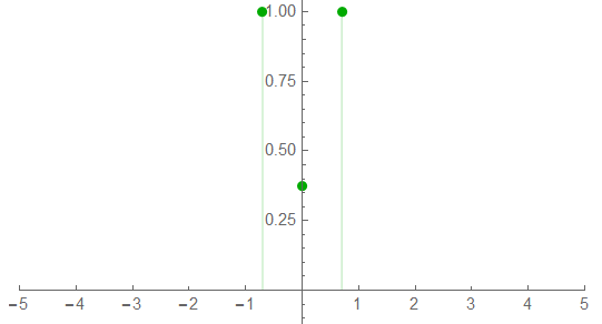
The full spectrum:

The phase spectrum:

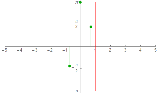
The half-spectrum shows energy at DC; the signal is under-sampled. The frequency resolution is about 0.5Hz.

I once worked on a project where the sample frequency was 2 with a signal bandwidth of 0.1 to 1.0. The filter had a corner frequency of 1; an 8th-order filter was not sufficient to provide the desired amplitude measurement accuracy of 0.25%.

The solution? “An algorithm will correct for the error“.

Could be, I’m not a DSP expert.

Page 5
Page 7

Lots of plots here … more than enough for one session, so

That’s good for now …